Glimepiride whole-body PBPK (Elias 2025)
Source:vignettes/articles/Elias_2025_glimepiride_pbpk.Rmd
Elias_2025_glimepiride_pbpk.RmdThe model
Elias_2025_glimepiride_pbpk is the whole-body
physiologically based pharmacokinetic model that Elias and Koenig (2025)
built as a “digital twin” of the sulfonylurea glimepiride from 20
curated clinical studies, and distributed as SBML under CC-BY. It tracks
the parent drug and its two sequential metabolites: M1
(cyclohexylhydroxymethyl-glimepiride, formed by CYP2C9 and about 30% as
active as the parent) and M2 (carboxy-glimepiride).
mod <- rxode2::rxode(readModelDb("Elias_2025_glimepiride_pbpk"))
length(mod$state)
#> [1] 47
The 41 ODEs are organised as a systemic circulation (venous, arterial, portal and hepatic-venous plasma pools, plus lung and a lumped rest-of-body tissue) linking three submodels (paper Figure 1, Supplementary Figure S2):
-
Intestine. Oral glimepiride dissolves from the dose
compartment into the gut lumen (
ka_dis_gli) and is absorbed first order into gut plasma (gliabs_k). M1 and M2 pass from gut plasma back into the lumen (mreabs_k) and leave in feces (mexc_k). -
Liver. Glimepiride equilibrates rapidly between
liver plasma and tissue (
gliim_k), is converted to M1 by CYP2C9 (Michaelis-Menten), and M1 is converted to M2 (first order). Both metabolites are exported back to plasma. - Kidney. M1 and M2 are excreted in urine first order from kidney plasma. Unchanged glimepiride is not excreted renally.
Lung and rest-of-body tissue take up all three species through one
shared partition coefficient (kp_gli) and one shared
distribution rate (ftissue_gli).
A note on units and dosing. Following the source
SBML, every plasma and tissue state is a concentration in
mmol/L rather than an amount; only the dosing compartments (mg) and the
cumulative urine and feces pools (mmol) are amounts. Give oral doses
into depot and intravenous doses into depot_iv
(glimepiride), depot_iv_m1 or depot_iv_m2,
never directly into a plasma or tissue compartment. Model time is in
minutes. The outputs Cc,
Cc_m1 and Cc_m2 are venous plasma
concentrations in umol/L; multiply by the molecular weight (490.616,
506.62 and 520.6 g/mol) to get ng/mL.
Population
pop <- mod$population
data.frame(Field = names(pop), Value = vapply(pop, as.character, character(1))) |>
knitr::kable(row.names = FALSE)| Field | Value |
|---|---|
| species | human |
| n_subjects | NA |
| n_studies | 20 |
| age_range | adults; pediatric studies excluded (Methods Section 4.1) |
| weight_range | 75 kg reference individual; 40-170 kg explored in the body-weight scan (Figure 5) |
| sex_female_pct | NA |
| disease_state | Healthy volunteers, patients with type 2 diabetes mellitus, subjects with renal impairment, normal-weight and morbidly obese subjects, and carriers of CYP2C9 1, 2 and *3 alleles (Table 1). Hepatic impairment was simulated from the cirrhosis model with limited clinical comparison data. |
| dose_range | Oral 0.5-8 mg single and multiple dose; intravenous glimepiride 0.25-1.5 mg and intravenous M1 1.5 mg (Table 1). |
| regions | Europe, East Asia, Egypt and the USA across the curated studies (Table 1 and Supplementary Section S6) |
| notes | Deterministic typical-individual model. The paper reports a single optimized parameter set (Supplementary Table S1), used for every simulation without refitting, and no inter-individual variability or residual-error model; the only stochastic element in the paper is the lognormal sampling of CYP2C9 activity in the population analyses. Parameters were fitted by weighted least squares (100 local-optimisation runs) to the healthy, fasted subset of the curated PK-DB dataset (Methods Section 4.3). |
The model was fitted to the healthy, fasted subset of 20 curated clinical studies (paper Table 1): healthy volunteers, patients with type 2 diabetes, subjects with renal impairment, normal-weight and morbidly obese subjects, and carriers of CYP2C9 1, 2 and *3 alleles, with oral doses of 0.5-8 mg and intravenous glimepiride (0.25-1.5 mg) or M1 (1.5 mg). It is a deterministic typical-individual model: the authors report one optimized parameter set (Supplementary Table S1) and no between-subject variability or residual error. The reference individual weighs 75 kg.
Source trace
Every value in ini() traces to the manuscript Methods,
the Supplementary Materials (equations in Section S3, optimized
parameters in Table S1), or the authors’ archived SBML model, which the
manuscript names as the definitive model source.
| Quantity | Parameters | Source |
|---|---|---|
| Fractional organ and blood-pool volumes |
fvar, fvgu, fvhv,
fvki, fvli, fvlu,
fvpo, fvve
|
Archived SBML FV* (not printed in the paper) |
| Fractional blood flows |
fqgu, fqh, fqki,
fqlu
|
Archived SBML FQ*
|
| Cardiac output, hematocrit, blood fraction |
covbw, fcardio, hct,
fblood
|
Archived SBML COBW, f_cardiac_function,
HCT, Fblood
|
| Molecular weights |
mr_gli, mr_m1, mr_m2
|
Archived SBML Mr_gli, Mr_m1,
Mr_m2
|
| Partition coefficient, tissue distribution |
kp_gli, ftissue_gli
|
Table S1 (10.02060; 0.00071 L/min) |
| Dissolution | ka_dis_gli |
Section S3 names it; value 2 /h from the archived SBML |
| Absorption, food scaling |
gliabs_k, f_absorption
|
Table S1 (0.01590 /min); f_absorption = 1 (fasted) |
| Intestinal metabolite handling |
mreabs_k, mexc_k
|
Table S1 (0.01592; 0.00017 /min) |
| Hepatic import | gliim_k |
Section S3 names it; value 100 /min from the archived SBML (not optimized) |
| CYP2C9 conversion GLI -> M1 |
gli2m1_vmax, gli2m1_km_gli
|
Table S1 (Vmax 0.00005 mmol/min/L); Km 2.25 umol/L from the archived SBML, literature-based per Methods 4.2 |
| M1 -> M2, metabolite export |
m12m2_k, m1ex_li_k,
m2ex_li_k
|
Table S1 (0.01485; 0.07774; 99.99817 /min) |
| Urinary excretion |
m1ex_ki_k, m2ex_ki_k
|
Table S1 (0.14801; 0.09849 /min) |
| Intravenous release | ti_iv |
Archived SBML ti_gli (10 s) |
| Scenario covariates |
WT, RENALFUNC_REL,
HEPFUNC_REL, CYP2C9
|
Methods 4.2 (KDIGO, Child-Turcotte-Pugh and CYP2C9 allele mappings); Supplementary Table S2 |
The intestine, kidney and liver rate laws are Supplementary Section
S3. The whole-body circulation ODEs are not written out anywhere
in the manuscript or supplement and were taken from the
archived SBML (models/glimepiride_body_flat.md, Zenodo 10.5281/zenodo.15189579,
version 0.6.1, the version Methods 4.2 names). That archive’s optimized
parameters agree with Supplementary Table S1 to every printed digit.
Simulation helper
mw <- c(gli = 490.616, m1 = 506.62, m2 = 520.6)

# One event table for any number of subjects. Observations sit on the `venous`
# ODE state; rxode2 returns the algebraic outputs (Cc, Cc_m1, Cc_m2,
# Aurine_m1m2, ...) as columns on those rows. Time is in minutes.
sim_gli <- function(subjects, hours = 48, by_min = 15) {
  tt <- seq(0, hours * 60, by = by_min)
  ev <- bind_rows(lapply(seq_len(nrow(subjects)), function(i) {
    s <- subjects[i, ]
    bind_rows(
      data.frame(id = i, time = 0, amt = s$amt, evid = 1L, cmt = s$route),
      data.frame(id = i, time = tt, amt = 0, evid = 0L, cmt = "venous")
    ) |>
      mutate(WT = s$WT, RENALFUNC_REL = s$RENALFUNC_REL,
             HEPFUNC_REL = s$HEPFUNC_REL, CYP2C9 = s$CYP2C9)
  }))
  # The model has no etas, so rxode2 warns that a multi-subject solve has no
  # omega; every subject is a deterministic scenario, which is intended.
  out <- withCallingHandlers(
    rxode2::rxSolve(mod, ev, returnType = "data.frame",
                    atol = 1e-12, rtol = 1e-10),
    warning = function(w) {
      if (grepl("without 'omega'", conditionMessage(w), fixed = TRUE)) {
        invokeRestart("muffleWarning")
      }
    }
  )
  # rxode2 drops the id column when only one subject is solved.
  if (!"id" %in% names(out)) out$id <- 1L
  out |>
    left_join(mutate(subjects, id = seq_len(n())), by = "id",
              suffix = c("", ".cov")) |>
    mutate(hour = time / 60)
}

subject <- function(amt, route = "depot", WT = 75, RENALFUNC_REL = 1,
                    HEPFUNC_REL = 1, CYP2C9 = 1, label = NA_character_) {
  data.frame(amt = amt, route = route, WT = WT, RENALFUNC_REL = RENALFUNC_REL,
             HEPFUNC_REL = HEPFUNC_REL, CYP2C9 = CYP2C9, label = label)
}

auc_trap <- function(t, y) sum(diff(t) * (head(y, -1) + tail(y, -1)) / 2)
Agreement with the authors’ SBML
The decisive check is that this translation reproduces the authors’
own model. The maintainers simulated the archived SBML
(glimepiride_body_flat.xml, v0.6.1) in libroadrunner 2.11.0
for nine scenarios covering every dosing route and every scenario
covariate, and recorded the 0-48 h maximum venous concentration of each
species (on a 15-minute grid) and the 48-hour cumulative urinary
recovery of M1 + M2. The same scenarios are solved here.
sbml_ref <- tibble::tribble(
  ~label,              ~cmax_gli, ~cmax_m1,  ~cmax_m2,   ~urine48,
  "PO 4 mg",             0.61412,  0.13026,  0.065808,    3.9265,
  "PO 1 mg",             0.14649,  0.036309, 0.017927,    1.0017,
  "PO 8 mg",             1.2877,   0.22697,  0.11761,     7.6442,
  "IV 1 mg",             0.27741,  0.043921, 0.01975,     0.99554,
  "IV M1 1.5 mg",        0,        0.3795,   0.038029,    1.8036,
  "PO 1 mg, CTP C",      0.23333,  0.01294,  0.0038541,   0.54932,
  "PO 3 mg, severe RI",  0.45403,  0.14468,  0.085931,    1.0733,
  "PO 4 mg, *3/*3",      0.80087,  0.039058, 0.021142,    2.2659,
  "PO 8 mg, 120 kg",     0.81921,  0.17192,  0.091591,    8.5573
)

scen <- bind_rows(
  subject(4, label = "PO 4 mg"),
  subject(1, label = "PO 1 mg"),
  subject(8, label = "PO 8 mg"),
  subject(1, route = "depot_iv", label = "IV 1 mg"),
  subject(1.5, route = "depot_iv_m1", label = "IV M1 1.5 mg"),
  subject(1, HEPFUNC_REL = 1 - 0.8127551020408164, label = "PO 1 mg, CTP C"),
  subject(3, RENALFUNC_REL = 0.19, label = "PO 3 mg, severe RI"),
  subject(4, CYP2C9 = 0.23, label = "PO 4 mg, *3/*3"),
  subject(8, WT = 120, label = "PO 8 mg, 120 kg")
)
sim_scen <- sim_gli(scen)

ours <- sim_scen |>
  group_by(label) |>
  summarise(cmax_gli = max(Cc), cmax_m1 = max(Cc_m1), cmax_m2 = max(Cc_m2),
            urine48 = 1000 * Aurine_m1m2[which.max(time)], .groups = "drop")

cmp <- inner_join(sbml_ref, ours, by = "label", suffix = c("_sbml", "_rx"))
rel_diff <- function(a, b) ifelse(b == 0, abs(a), abs(a - b) / b)
cmp <- cmp |>
  mutate(
    d_gli = rel_diff(cmax_gli_rx, cmax_gli_sbml),
    d_m1 = rel_diff(cmax_m1_rx, cmax_m1_sbml),
    d_m2 = rel_diff(cmax_m2_rx, cmax_m2_sbml),
    d_urine = rel_diff(urine48_rx, urine48_sbml)
  )

cmp |>
  select(label, cmax_gli_sbml, cmax_gli_rx, cmax_m1_sbml, cmax_m1_rx,
         urine48_sbml, urine48_rx) |>
  rename("Scenario" = label,
         "GLI Cmax, SBML (umol/L)" = cmax_gli_sbml,
         "GLI Cmax, nlmixr2lib (umol/L)" = cmax_gli_rx,
         "M1 Cmax, SBML (umol/L)" = cmax_m1_sbml,
         "M1 Cmax, nlmixr2lib (umol/L)" = cmax_m1_rx,
         "M1+M2 urine 48 h, SBML (umol)" = urine48_sbml,
         "M1+M2 urine 48 h, nlmixr2lib (umol)" = urine48_rx) |>
knitr::kable(digits = 4)| Scenario | GLI Cmax, SBML (umol/L) | GLI Cmax, nlmixr2lib (umol/L) | M1 Cmax, SBML (umol/L) | M1 Cmax, nlmixr2lib (umol/L) | M1+M2 urine 48 h, SBML (umol) | M1+M2 urine 48 h, nlmixr2lib (umol) |
|---|---|---|---|---|---|---|
| PO 4 mg | 0.6141 | 0.6141 | 0.1303 | 0.1303 | 3.9265 | 3.9265 |
| PO 1 mg | 0.1465 | 0.1465 | 0.0363 | 0.0363 | 1.0017 | 1.0017 |
| PO 8 mg | 1.2877 | 1.2877 | 0.2270 | 0.2270 | 7.6442 | 7.6443 |
| IV 1 mg | 0.2774 | 0.2774 | 0.0439 | 0.0439 | 0.9955 | 0.9955 |
| IV M1 1.5 mg | 0.0000 | 0.0000 | 0.3795 | 0.3795 | 1.8036 | 1.8037 |
| PO 1 mg, CTP C | 0.2333 | 0.2333 | 0.0129 | 0.0129 | 0.5493 | 0.5493 |
| PO 3 mg, severe RI | 0.4540 | 0.4540 | 0.1447 | 0.1447 | 1.0733 | 1.0733 |
| PO 4 mg, 3/3 | 0.8009 | 0.8009 | 0.0391 | 0.0391 | 2.2659 | 2.2659 |
| PO 8 mg, 120 kg | 0.8192 | 0.8192 | 0.1719 | 0.1719 | 8.5573 | 8.5573 |
# The two sides solve the same equations with the same parameters (here
# rounded to 5 significant digits), so the only difference is numerical; a
# transcription error in any rate law moves at least one of these columns by
# whole percent.
stopifnot(max(cmp$d_gli, cmp$d_m1, cmp$d_m2, cmp$d_urine) < 1e-3)
Dose dependency (Figure 2)
doses <- c(1, 2, 3, 4, 6, 8)
sim_dose <- sim_gli(bind_rows(lapply(doses, function(d) subject(d, label = paste(d, "mg")))),
                    hours = 24, by_min = 5)

sim_dose |>
  tidyr::pivot_longer(c(Cc, Cc_m1, Cc_m2), names_to = "species", values_to = "conc") |>
  mutate(species = recode(species, Cc = "Glimepiride", Cc_m1 = "M1", Cc_m2 = "M2"),
         dose = factor(amt)) |>
  ggplot(aes(hour, conc, colour = dose)) +
  geom_line() +
  facet_wrap(~species, scales = "free_y") +
  labs(x = "Time (h)", y = "Plasma concentration (umol/L)", colour = "Dose (mg)",
       caption = "Replicates Figure 2B/Supplementary Figure S4 of Elias 2025 (typical 75 kg individual).")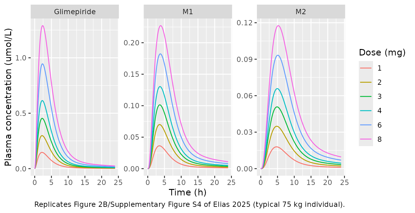
dose_tab <- sim_dose |>
  group_by(amt) |>
  summarise(
    cmax_ng = max(Cc) * mw[["gli"]],
    tmax_h = hour[which.max(Cc)],
    auc24_ng = auc_trap(hour, Cc * mw[["gli"]]),
    cmax_m1_ng = max(Cc_m1) * mw[["m1"]],
    cmax_m2_ng = max(Cc_m2) * mw[["m2"]],
    .groups = "drop"
  ) |>
  mutate(cmax_per_mg = cmax_ng / amt, auc_per_mg = auc24_ng / amt)

dose_tab |>
  rename("Dose (mg)" = amt, "GLI Cmax (ng/mL)" = cmax_ng, "GLI tmax (h)" = tmax_h,
         "GLI AUC0-24 (ng*h/mL)" = auc24_ng, "M1 Cmax (ng/mL)" = cmax_m1_ng,
         "M2 Cmax (ng/mL)" = cmax_m2_ng, "Cmax / dose" = cmax_per_mg,
         "AUC0-24 / dose" = auc_per_mg) |>
knitr::kable(digits = 2)| Dose (mg) | GLI Cmax (ng/mL) | GLI tmax (h) | GLI AUC0-24 (ng*h/mL) | M1 Cmax (ng/mL) | M2 Cmax (ng/mL) | Cmax / dose | AUC0-24 / dose |
|---|---|---|---|---|---|---|---|
| 1 | 71.95 | 2.17 | 373.41 | 18.40 | 9.33 | 71.95 | 373.41 |
| 2 | 146.22 | 2.17 | 770.07 | 35.47 | 18.14 | 73.11 | 385.04 |
| 3 | 222.75 | 2.25 | 1189.86 | 51.33 | 26.44 | 74.25 | 396.62 |
| 4 | 301.29 | 2.25 | 1632.55 | 66.05 | 34.27 | 75.32 | 408.14 |
| 6 | 463.94 | 2.33 | 2585.28 | 92.37 | 48.56 | 77.32 | 430.88 |
| 8 | 632.94 | 2.33 | 3624.92 | 115.08 | 61.22 | 79.12 | 453.11 |
urine_8mg <- 1000 * sim_gli(subject(8), hours = 48)$Aurine_m1m2 |> max()
urine_8mg
#> [1] 7.644275
Section 2.3 reports Tmax “stable at 2.0-2.5 h”, Cmax and AUC increasing proportionally with dose, and cumulative M1 + M2 urinary excretion “reaching about 7 umol by 48 h for the 8 mg dose”. Figure 2C’s simulated line passes about 640 ng/mL at 8 mg (the text’s “700 ng/mL” is the line’s end beyond the last dose). Glimepiride conversion to M1 is Michaelis-Menten, so exposure is very slightly more than dose-proportional, as Figure 2C also shows.
Renal impairment (Figure 3)
Methods 4.2 maps the KDIGO categories onto
RENALFUNC_REL: normal 1.0, mild 0.69, moderate 0.32, severe
0.19. Renal function scales only the urinary excretion of M1 and M2.
renal_levels <- c(Normal = 1, Mild = 0.69, Moderate = 0.32, Severe = 0.19)
sim_renal <- sim_gli(bind_rows(lapply(names(renal_levels), function(n)
  subject(3, RENALFUNC_REL = renal_levels[[n]], label = n))))
sim_renal$label <- factor(sim_renal$label, levels = names(renal_levels))

sim_renal |>
  mutate(`M1 + M2 urine (umol)` = 1000 * Aurine_m1m2,
         `M1 plasma (umol/L)` = Cc_m1) |>
  tidyr::pivot_longer(c(`M1 plasma (umol/L)`, `M1 + M2 urine (umol)`)) |>
  ggplot(aes(hour, value, colour = label)) +
  geom_line() +
  facet_wrap(~name, scales = "free_y") +
  labs(x = "Time (h)", y = NULL, colour = "Renal function",
       caption = "Replicates Figure 3B of Elias 2025 (3 mg oral).")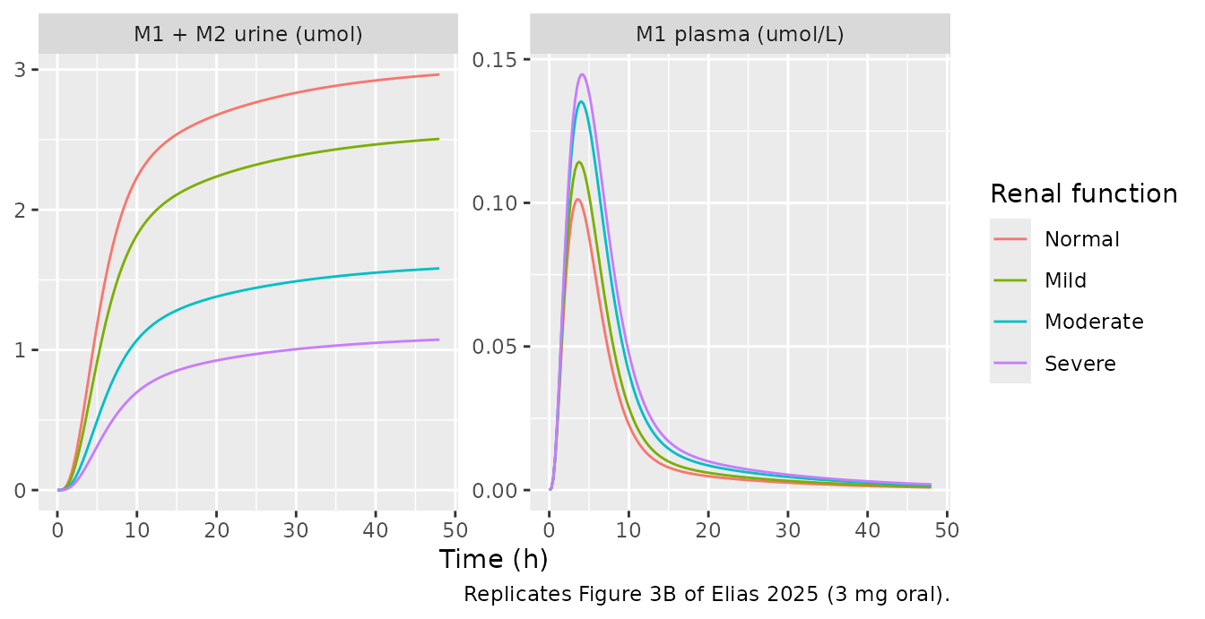
renal_tab <- sim_renal |>
  group_by(label) |>
  summarise(cmax_gli = max(Cc), auc_m1 = auc_trap(hour, Cc_m1),
            urine48 = 1000 * max(Aurine_m1m2), .groups = "drop")
knitr::kable(renal_tab |>
  rename("Renal function" = label, "GLI Cmax (umol/L)" = cmax_gli,
         "M1 AUC0-48 (umol*h/L)" = auc_m1, "M1+M2 urine 48 h (umol)" = urine48),
digits = 3)| Renal function | GLI Cmax (umol/L) | M1 AUC0-48 (umol*h/L) | M1+M2 urine 48 h (umol) |
|---|---|---|---|
| Normal | 0.454 | 0.747 | 2.965 |
| Mild | 0.454 | 0.879 | 2.505 |
| Moderate | 0.454 | 1.123 | 1.581 |
| Severe | 0.454 | 1.246 | 1.073 |
Section 2.4: parent exposure is unchanged, metabolites accumulate, and the 48-hour urinary recovery falls from about 3 umol (normal) to about 1 umol (severe impairment) after 3 mg.
Hepatic impairment (Figure 4)
The cirrhosis severity f_cirrhosis of the source is
1 - HEPFUNC_REL. The authors’ archived scenarios use
f_cirrhosis = 0.3995 (CTP A), 0.6980 (CTP B) and 0.8128
(CTP C), following Koeller et al. (2021).
cirr_levels <- c(Control = 0, `CTP A` = 0.3994897959183674,
                 `CTP B` = 0.6979591836734694, `CTP C` = 0.8127551020408164)
sim_hep <- sim_gli(bind_rows(lapply(names(cirr_levels), function(n)
  subject(1, HEPFUNC_REL = 1 - cirr_levels[[n]], label = n))))
sim_hep$label <- factor(sim_hep$label, levels = names(cirr_levels))

sim_hep |>
  tidyr::pivot_longer(c(Cc, Cc_m1)) |>
  mutate(name = recode(name, Cc = "Glimepiride", Cc_m1 = "M1")) |>
  ggplot(aes(hour, value, colour = label)) +
  geom_line() +
  facet_wrap(~name, scales = "free_y") +
  labs(x = "Time (h)", y = "Plasma concentration (umol/L)", colour = NULL,
       caption = "Replicates Figure 4B of Elias 2025 (1 mg oral).")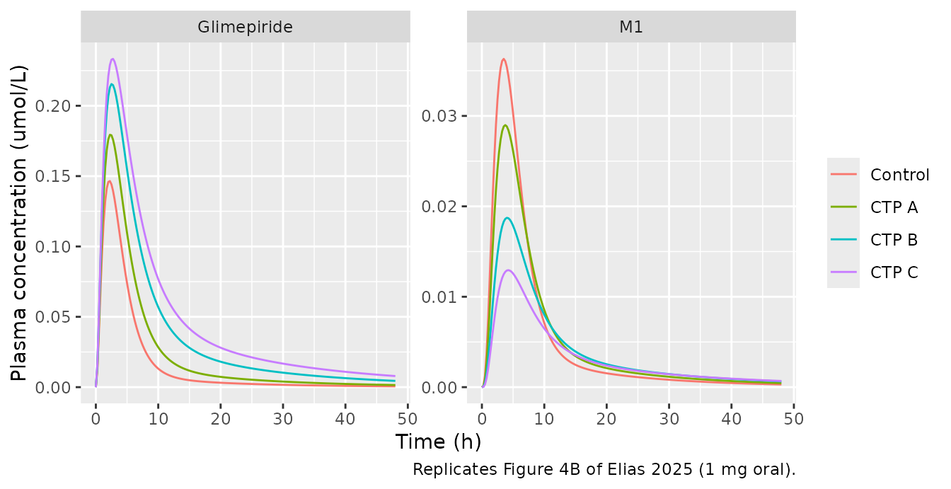
hep_tab <- sim_hep |>
  group_by(label) |>
  summarise(cmax_ng = max(Cc) * mw[["gli"]], auc48 = auc_trap(hour, Cc * mw[["gli"]]),
            cmax_m1 = max(Cc_m1), .groups = "drop") |>
  mutate(auc_ratio = auc48 / auc48[1])
knitr::kable(hep_tab |>
  rename("Liver function" = label, "GLI Cmax (ng/mL)" = cmax_ng,
         "GLI AUC0-48 (ng*h/mL)" = auc48, "M1 Cmax (umol/L)" = cmax_m1,
         "AUC ratio vs control" = auc_ratio),
digits = 2)| Liver function | GLI Cmax (ng/mL) | GLI AUC0-48 (ng*h/mL) | M1 Cmax (umol/L) | AUC ratio vs control |
|---|---|---|---|---|
| Control | 71.87 | 388.40 | 0.04 | 1.00 |
| CTP A | 88.00 | 584.24 | 0.03 | 1.50 |
| CTP B | 105.69 | 916.02 | 0.02 | 2.36 |
| CTP C | 114.47 | 1159.27 | 0.01 | 2.98 |
Section 2.5: Cmax “nearly doubled from 75 ng/mL in normal function to 125 ng/mL in severe cirrhosis, while AUC increased … by approximately 3.5-fold”, and metabolite concentrations fall.
Body weight (Figure 5)
bws <- c(40, 55, 72, 100, 130, 170)
sim_bw <- sim_gli(bind_rows(lapply(bws, function(w) subject(8, WT = w, label = paste(w, "kg")))))
bw_tab <- sim_bw |>
  group_by(WT) |>
  summarise(cmax_ng = max(Cc) * mw[["gli"]], cmax_um = max(Cc),
            auc48 = auc_trap(hour, Cc * mw[["gli"]]),
            tmax_h = hour[which.max(Cc)], .groups = "drop")

ggplot(bw_tab, aes(WT, cmax_ng)) +
  geom_line() + geom_point() +
  labs(x = "Body weight (kg)", y = "Glimepiride Cmax (ng/mL)",
       caption = "Replicates Figure 5C (Cmax panel) of Elias 2025 (8 mg oral).")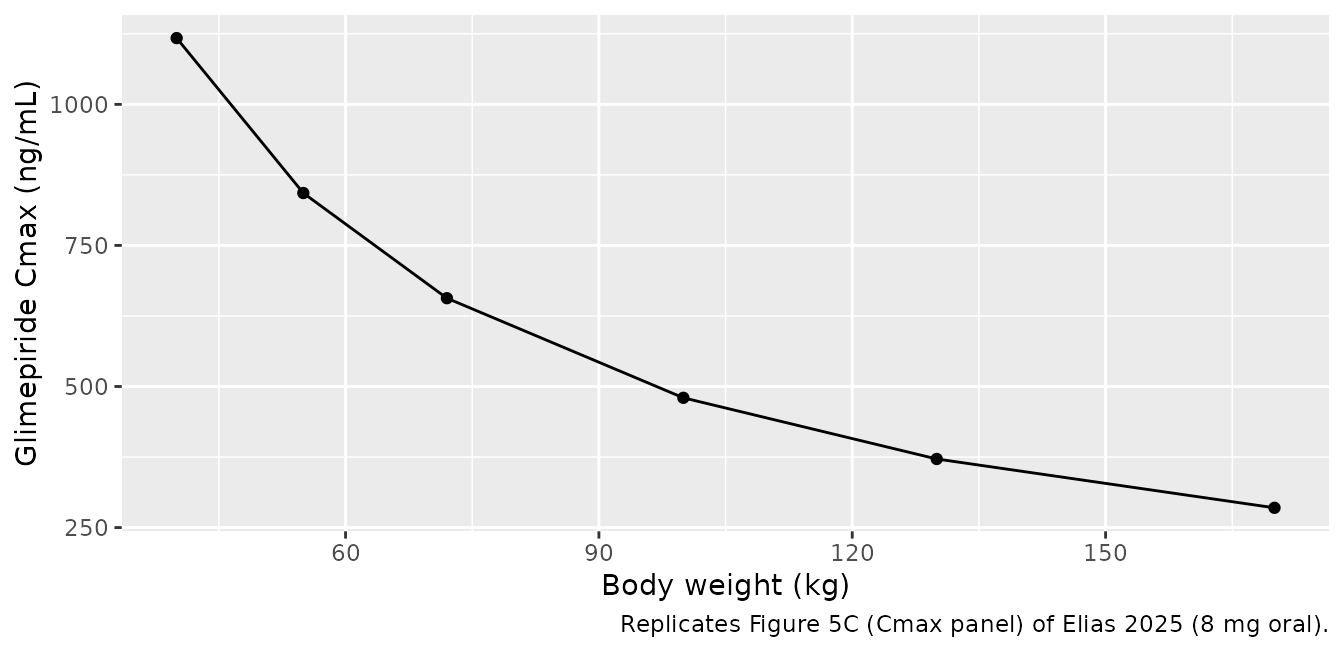
knitr::kable(bw_tab |>
  rename("Body weight (kg)" = WT, "GLI Cmax (ng/mL)" = cmax_ng,
         "GLI Cmax (umol/L)" = cmax_um, "GLI AUC0-48 (ng*h/mL)" = auc48,
         "GLI tmax (h)" = tmax_h),
digits = 2)| Body weight (kg) | GLI Cmax (ng/mL) | GLI Cmax (umol/L) | GLI AUC0-48 (ng*h/mL) | GLI tmax (h) |
|---|---|---|---|---|
| 40 | 1117.44 | 2.28 | 6712.57 | 2.25 |
| 55 | 842.84 | 1.72 | 5069.80 | 2.25 |
| 72 | 656.51 | 1.34 | 3928.12 | 2.25 |
| 100 | 479.96 | 0.98 | 2834.12 | 2.50 |
| 130 | 371.56 | 0.76 | 2168.80 | 2.50 |
| 170 | 285.02 | 0.58 | 1645.74 | 2.50 |
Section 2.6: Cmax falls from about 1,000 ng/mL at 40 kg to 300 ng/mL at 170 kg and AUC from about 6,000 to 2,000 ng*h/mL, with Tmax stable. For the Shukla 2004 cohorts (72 kg and 130 kg in the authors’ simulation set-up) the text quotes peaks of “1.4” and “0.8”; Figure 5B shows these are umol/L, not ug/mL.
CYP2C9 genotype (Figure 6)
Allele activities are 1 = 1.00, 2 = 0.68, *3 = 0.23 (Supplementary Table S2), and the diplotype activity is the mean of the two alleles.
allele <- c(`*1` = 1, `*2` = 0.68, `*3` = 0.23)
genotypes <- c("*1/*1", "*1/*2", "*1/*3", "*3/*3")
geno_act <- sapply(strsplit(genotypes, "/"), function(a) mean(allele[a]))
names(geno_act) <- genotypes
geno_act
#> *1/*1 *1/*2 *1/*3 *3/*3
#> 1.000 0.840 0.615 0.230

sim_cyp <- sim_gli(bind_rows(lapply(genotypes, function(g)
  subject(4, CYP2C9 = geno_act[[g]], label = g))))
sim_cyp$label <- factor(sim_cyp$label, levels = genotypes)

ggplot(sim_cyp, aes(hour, Cc, colour = label)) +
  geom_line() +
  labs(x = "Time (h)", y = "Glimepiride (umol/L)", colour = "CYP2C9",
       caption = "Replicates Figure 6B of Elias 2025 (4 mg oral, fixed activities).")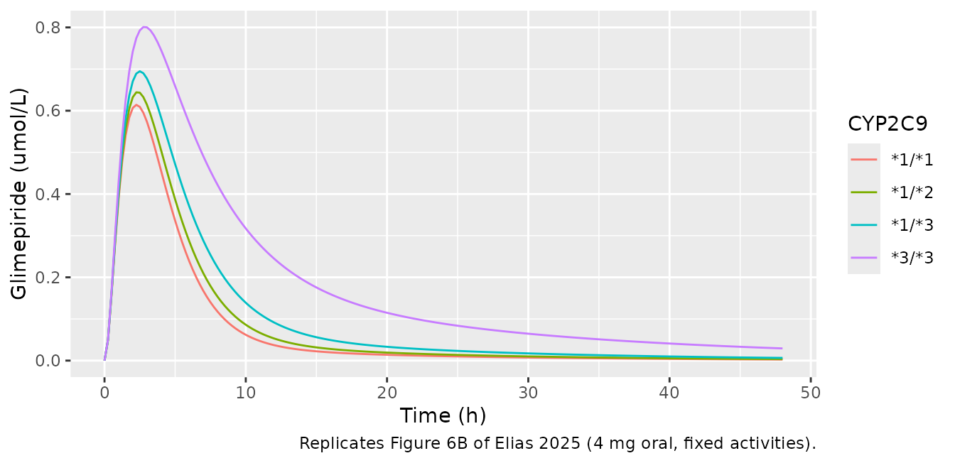
cyp_tab <- sim_cyp |>
  group_by(label) |>
  summarise(auc48 = auc_trap(hour, Cc * mw[["gli"]]), .groups = "drop") |>
  mutate(ratio = auc48 / auc48[1])
cyp_tab
#> # A tibble: 4 × 3
#>   label auc48 ratio
#>   <fct> <dbl> <dbl>
#> 1 *1/*1 1699.  1
#> 2 *1/*2 1955.  1.15
#> 3 *1/*3 2473.  1.46
#> 4 *3/*3 4382.  2.58

stopifnot(
  isTRUE(all.equal(unname(geno_act), c(1, 0.84, 0.615, 0.23))),
  all(diff(cyp_tab$auc48) > 0),
  # "approximately two-fold" (Discussion) to "up to 2.5-fold" (Section 2.7);
  # the 0-48 h ratio of the typical individual is about 2.6.
  cyp_tab$ratio[4] > 1.8, cyp_tab$ratio[4] < 2.8
)
Probabilistic CYP2C9 activity
For the population analyses each allele activity was drawn from a lognormal distribution with shape sigma = 0.81 (fitted to diclofenac intrinsic clearance in human liver microsomes, Supplementary Table S4) scaled so that its mean is the allele activity; the diplotype activity is the mean of the two draws. Reproducing the genotype medians of Supplementary Table S5 checks that reading.
set.seed(20251006)
draw_geno <- function(g, n) {
  a <- strsplit(g, "/")[[1]]
  draw <- function(m) rlnorm(n, meanlog = log(m) - 0.81^2 / 2, sdlog = 0.81)
  (draw(allele[[a[1]]]) + draw(allele[[a[2]]])) / 2
}
big <- sapply(genotypes, draw_geno, n = 1e5)
act_tab <- data.frame(genotype = genotypes, mean = colMeans(big),
                      median = apply(big, 2, median))
act_tab$median_tableS5 <- c(0.83, 0.70, 0.48, 0.19)
knitr::kable(act_tab |> rename("Genotype" = genotype, "Mean" = mean,
                               "Median" = median, "Table S5 median" = median_tableS5),
digits = 3)| Genotype | Mean | Median | Table S5 median | |
|---|---|---|---|---|
| 1/1 | 1/1 | 1.001 | 0.829 | 0.83 |
| 1/2 | 1/2 | 0.840 | 0.691 | 0.70 |
| 1/3 | 1/3 | 0.612 | 0.480 | 0.48 |
| 3/3 | 3/3 | 0.229 | 0.190 | 0.19 |
A virtual cohort of 150 subjects per genotype (4 mg oral, 75 kg) then gives the distribution of glimepiride exposure, which the NCA below compares with Supplementary Table S6.
n_per <- 150
cohort <- bind_rows(lapply(genotypes, function(g)
  data.frame(genotype = g, CYP2C9 = draw_geno(g, n_per))))
sim_pop <- sim_gli(
  bind_rows(lapply(seq_len(nrow(cohort)), function(i)
    subject(4, CYP2C9 = cohort$CYP2C9[i], label = cohort$genotype[i]))),
  hours = 24, by_min = 15
)
sim_pop$genotype <- factor(sim_pop$label, levels = genotypes)

sim_pop |>
  group_by(id, genotype) |>
  summarise(auc24 = auc_trap(hour, Cc * mw[["gli"]]), .groups = "drop") |>
  ggplot(aes(genotype, auc24, fill = genotype)) +
  geom_boxplot(show.legend = FALSE) +
  labs(x = "CYP2C9 genotype", y = "Glimepiride AUC0-24 (ng*h/mL)",
       caption = "Replicates Figure 6D (AUC panel) of Elias 2025.")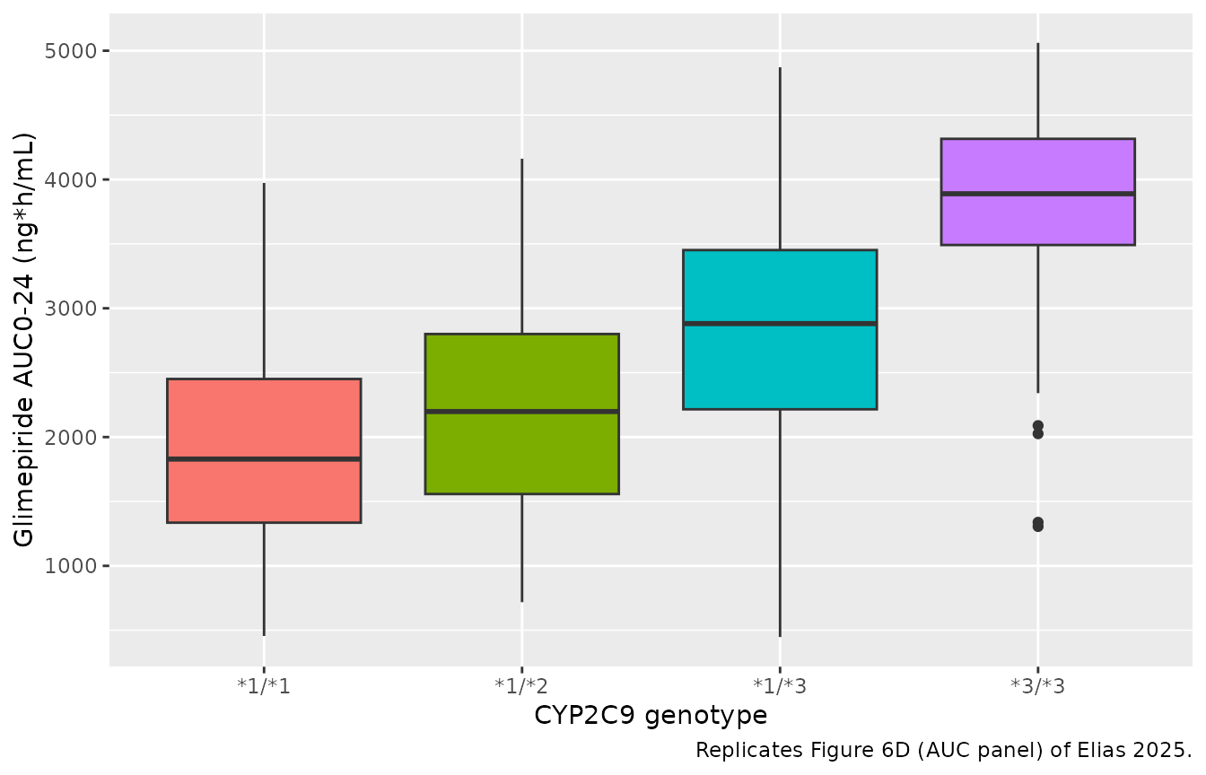
Non-compartmental analysis
PKNCA on the probabilistic cohort, grouped by genotype, against the genotype medians of Supplementary Table S6 (4 mg oral; Cmax converted from umol/L to ng/mL). Table S6 does not state its AUC interval. Its AUC values match the 0-24 h AUC of this cohort – medians, upper quartiles and maxima alike, the maxima levelling off near 5,000 ng*h/mL for every genotype as a truncated AUC does – and fall 20-30% short of AUC0-inf for the low-activity genotypes, whose terminal phase is longest, so the comparison uses AUC0-24.
conc <- sim_pop |>
  filter(!is.na(Cc)) |>
  transmute(id, genotype, hour, conc = Cc * mw[["gli"]])
dose_df <- conc |>
  distinct(id, genotype) |>
  mutate(hour = 0, dose = 4)

o_conc <- PKNCA::PKNCAconc(as.data.frame(conc), conc ~ hour | genotype + id)
o_dose <- PKNCA::PKNCAdose(as.data.frame(dose_df), dose ~ hour | genotype + id)
nca <- PKNCA::pk.nca(PKNCA::PKNCAdata(
  o_conc, o_dose,
  intervals = data.frame(start = 0, end = 24, cmax = TRUE, tmax = TRUE,
                         auclast = TRUE)
))

ref_s6 <- data.frame(
  genotype = genotypes,
  cmax = c(0.645, 0.677, 0.724, 0.809) * mw[["gli"]],
  tmax = c(2.35, 2.44, 2.58, 2.88),
  auclast = c(1864.73, 2145.33, 2644.96, 3933.03)
)

nca_cmp <- nlmixr2lib::ncaComparisonTable(
  nca, ref_s6,
  by = "genotype",
  units = c(cmax = "ng/mL", tmax = "h", auclast = "ng*h/mL")
)
knitr::kable(nca_cmp)| NCA parameter | genotype | Reference | Simulated | % diff |
|---|---|---|---|---|
| Cmax (ng/mL) | 1/1 | 316 | 314 | -0.8% |
| Cmax (ng/mL) | 1/2 | 332 | 335 | +0.9% |
| Cmax (ng/mL) | 1/3 | 355 | 364 | +2.6% |
| Cmax (ng/mL) | 3/3 | 397 | 396 | -0.2% |
| Tmax (h) | 1/1 | 2.35 | 2.25 | -4.3% |
| Tmax (h) | 1/2 | 2.44 | 2.5 | +2.5% |
| Tmax (h) | 1/3 | 2.58 | 2.75 | +6.6% |
| Tmax (h) | 3/3 | 2.88 | 3 | +4.2% |
| AUClast (ng*h/mL) | 1/1 | 1860 | 1830 | -1.9% |
| AUClast (ng*h/mL) | 1/2 | 2150 | 2200 | +2.4% |
| AUClast (ng*h/mL) | 1/3 | 2640 | 2880 | +8.9% |
| AUClast (ng*h/mL) | 3/3 | 3930 | 3890 | -1.1% |
attr(nca_cmp, "footnote")
#> NULL

nca_med <- as.data.frame(nca$result) |>
  group_by(genotype, PPTESTCD) |>
  summarise(med = median(PPORRES), .groups = "drop") |>
  tidyr::pivot_wider(names_from = PPTESTCD, values_from = med) |>
  mutate(genotype = as.character(genotype)) |>
  inner_join(ref_s6, by = "genotype", suffix = c("_sim", "_ref"))

stopifnot(
  all(abs(nca_med$cmax_sim / nca_med$cmax_ref - 1) < 0.10),
  all(abs(nca_med$tmax_sim - nca_med$tmax_ref) <= 0.5),
  all(abs(nca_med$auclast_sim / nca_med$auclast_ref - 1) < 0.15)
)
Assumptions and deviations / Errata
- Whole-body ODEs and physiology from the archived SBML. The paper prints the submodel rate laws (Supplementary Section S3, partly as equation images) and the eleven optimized parameters (Table S1), but not the circulation ODEs, fractional organ volumes and blood flows, cardiac output, hematocrit, molecular weights, the dissolution rate (2 /h), the hepatic import rate (100 /min), the CYP2C9 Michaelis constant (2.25 umol/L) or the intravenous release time. These come from the authors’ archived SBML v0.6.1, which Methods 4.2 cites as the model (“version 0.6.1 (Elias and Koenig, 2025a)”). The archive’s optimized values agree with Table S1 to every printed digit.
-
Parameter precision. Table S1 prints three
parameters to only one or two significant digits
(
GLI2M1 Vmax0.00005,ftissue gli0.00071,MEXC k0.00017). The model uses the archive’s values (5.362e-5, 7.0864e-4, 1.7193e-4); the printed 0.00005 would lower the CYP2C9 Vmax by 7%. -
Deterministic model. No between-subject variability
or residual error is reported, so there are no etas and
propSdis fixed at zero. The probabilistic CYP2C9 analysis is reproduced in this vignette, outside the model, by drawing theCYP2C9covariate. - Lognormal CYP2C9 draws. The paper states the shape (0.81) and that the scale was “adjusted to match the mean activity of each allele”. Drawing each allele with mean equal to its activity reproduces the genotype means, medians and SDs of Supplementary Table S5 (e.g. 1/1 mean 1.00, median 0.83), confirming the reading. Table S5’s allele-level SD (0.73 for *1) does not match a sigma = 0.81 lognormal (which has CV 0.96); the genotype-level rows are reproduced and were used.
-
Renal scaling values. Methods 4.2 prints
f_renal_function= 0.69 / 0.32 / 0.19 for mild / moderate / severe impairment, and those values are used here. The authors’ archived scenario simulations use 0.495 / 0.347 / 0.198 instead (50, 35 and 20 of a 101 mL/min reference), and their Rosenkranz 1996 study simulation uses 0.5 / 0.35 / 0.2. Only metabolite exposure depends on this choice. -
Child-Turcotte-Pugh mapping. The paper does not
print the
f_cirrhosisvalues; 0.3995 / 0.6980 / 0.8128 for CTP A / B / C are the authors’ archived scenario values (following Koeller et al. 2021). - Body-weight peak units. Section 2.6 quotes Shukla 2004 peaks of “1.4 ug/mL” and “0.8 ug/mL”; Figure 5B shows them in umol/L, and the model reproduces them in umol/L.
-
Half-life. Rest-of-body tissue equilibrates slowly
(
ftissue_gli0.00071 L/min against a tissue volume of about 70 L with Kp 10), so the venous profile is multi-phasic and an NCA half-life depends on the fitting window. The paper’s “approximately 4 h” refers to the early elimination phase; it is not used as a gate here. -
Omitted SBML bookkeeping. The source carries states
with zero derivatives (
Afeces_gli,GU__gli_stomach), cumulative-infusion counters fed by zero-valued infusion-rate parameters (Ri_*,cum_dose_*) and a display-only creatinine-clearance output (KI__crcl, which needs height). None affects any concentration; they are omitted. Intravenous infusions can be given with an rxode2rateon thedepot_iv*compartments. -
Food effect.
f_absorptionscales the absorption rate; the paper gives no fed-state value, so it is held at 1 (fasted, the condition of the fitting data). - Table S6 AUC interval. The supplement does not say which AUC Table S6 reports. The 0-24 h AUC reproduces its genotype medians, quartiles and maxima; AUC0-inf does not for the 1/3 and 3/3 genotypes, so AUC0-24 is used in the comparison.
- Biogeographical populations (Figure 7) apply the same probabilistic CYP2C9 sampling with published genotype frequencies; they are not repeated here.