Apixaban (Ajavon-Hartmann 2025)
Source:vignettes/articles/AjavonHartmann_2025_apixaban.Rmd
AjavonHartmann_2025_apixaban.RmdModel and source
- Citation: Ajavon-Hartmann A, Jarugula P, Back H, Obianom O, Ludwig E, Crevar C, Marchisin D, Wang Z, Chen W, He B, Payne RM, Burns KM, Glatz AC, Male C, Monagle P, Perera V, Murthy B, Merali S. Characterization of Apixaban Pharmacokinetics/Pharmacodynamics and Dose Assessment in Pediatric Patients with Congenital or Acquired Heart Disease. Clin Pharmacol Ther. 2025;118:365-377. doi:10.1002/cpt.3689
- Description: Population PK model for oral apixaban in adults and pediatric patients, including children with congenital or acquired heart disease (SAXOPHONE) (Ajavon-Hartmann 2025): two-compartment with first-order absorption and elimination, dose-dependent relative bioavailability, body-weight power effects on CL/F and Vc/F, a fixed literature CYP maturation function on CL/F, age on Q/F, a 9-month-to-18-year age-group effect and an ALL/LL patient-type effect on ka, and a congenital-or-acquired-heart-disease effect on CL/F, with a zero-intercept linear mixed-effects PK/PD relationship to anti-factor Xa activity.
- Article: https://doi.org/10.1002/cpt.3689 (open access, PMC12272319)
- Supplement: Data S1 of the article (estimation methods, pediatric demographics, dataset composition, exposure summaries by age group, and the model-development schematic)
Ajavon-Hartmann 2025 added the sparse PK data of the phase II
SAXOPHONE trial (children aged 28 days to <18 years with congenital
or acquired heart disease, CAHD, needing chronic anticoagulation for
thromboembolism prevention) to the pooled adult and pediatric apixaban
population PK model. It then re-tested the patient-type covariates and
used the model to check the trial’s fixed-dose weight-tiered regimen
against adult exposure. The companion paper (Jarugula 2025,
Jarugula_2025_apixaban in this package) is the same model
fitted before the SAXOPHONE data were added. A zero-intercept linear
mixed-effects regression relates anti-factor Xa activity (AXA) to
apixaban concentration.
Compared with the Jarugula 2025 fit, backward elimination here kept the ALL/LL patient-type effect on ka, dropped it from Vc/F, and added a CAHD effect on CL/F (Figure S1 of the supplement).
Population
The final dataset held 6098 apixaban concentrations from 602 patients in 12 studies: 198 adults from eight adult studies, 56 pediatric patients at risk of venous or arterial thromboembolism from two phase I studies (CV185079, CV185118), 224 PREVAPIX-ALL patients with acute lymphoblastic leukemia or lymphoblastic lymphoma on asparaginase (CV185155), and 124 SAXOPHONE patients with CAHD (CV185362, 447 concentrations; Table S2). Table S1 describes the 404 pediatric patients: age 0.044 to 18 years (median 6.73), baseline weight 3 to 133 kg (median 22.6), 47.3% female, 78.5% White, 7.43% Asian and 6.44% Black. The SAXOPHONE patients were 0.378 to 18 years (median 7.5) and 6.1 to 133 kg (median 23.6); none was younger than 4 months. Adult demographics are not reported. The PK/PD analysis used 390 AXA values from 123 PREVAPIX-ALL and SAXOPHONE patients, measured with a drug-calibrated assay in ng/mL.
The same information is available programmatically via
readModelDb("AjavonHartmann_2025_apixaban")()$population.
Source trace
Each ini() entry carries an in-file comment naming its
source. The table collects them. The functional forms come from the
parameter-covariate equations under Table 1.
| Equation / parameter | Value | Source location |
|---|---|---|
lka (adult ka) |
log(0.525) 1/h | Table 1, theta1 |
lcl (CL/F, 67.4 kg, mature) |
log(4.7) L/h | Table 1, theta2 |
lvc (Vc/F, 67.4 kg) |
log(32.5) L | Table 1, theta3 |
lq (Q/F, 25 years) |
log(1.43) L/h | Table 1, theta4 |
lvp (Vp/F) |
log(20.8) L | Table 1, theta5 |
lgamma (F1 dose shape) |
log(0.89) | Table 1, theta6 |
logitifdepot50 (logit max F1 reduction) |
-0.457 | Table 1, theta7 |
e_wt_vc |
0.882 | Table 1, theta8 |
e_wt_cl |
0.68 | Table 1, theta9 |
e_age_q |
0.751 | Table 1, theta10 |
e_ped9m_ka |
1.23 | Table 1, theta11 |
lhill (ontogeny shape) |
log(0.83), fixed | Table 1, theta12 |
lpna50 (ontogeny AGE50) |
log(0.244) years, fixed | Table 1, theta13 |
e_form_capsule_fdepot |
1.1, fixed | Table 1, theta14 |
fbirth_cl |
0.05, fixed | Table 1, theta15 |
e_dis_all_ka |
-0.988 | Table 1, theta16 |
e_dis_heart_congenital_acquired_cl |
-0.185 | Table 1, theta17 |
etalka |
0.399 | Table 1, ZKA |
etalcl, etalvc, covariance |
0.149, 0.0719, 0.0838 | Table 1, ZCL, ZVC, ZVC:ZCL |
etalvp, etalq, covariance |
1.39, 0.989, 1.07 | Table 1, ZVP, ZQ, ZQ:ZVP |
expSd |
0.328 | Table 1, sigma 1,1 = 0.108 (SD 0.328), additive on log concentration |
slope_antiFXa |
0.916 | Table 3, slope |
etaslope_antiFXa |
0.0528^2 | Table 3, random-effect standard deviation 0.0528 |
addSd_antiFXa |
12.8 ng/mL | Table 3, residual 12.8 |
| ka equation | theta1 * (1 + PED9M * theta11) * exp(theta16 if PTYPE = ALL) |
Table 1 equations |
| CL/F equation incl. ontogeny | theta2 * (WT/67.4)^theta9 * MF * exp(theta17 if PTYPE = CAHD) |
Table 1 equations and MF footnote |
| Vc/F, Q/F, Vp/F equations | see model file | Table 1 equations |
| F1 equation | 1 for dose <= 2.5 mg, else
1 - expit(theta7) * ((DOSE - 2.5)/47.5)^theta6; times 1.1
for sprinkle capsule |
Table 1 equations |
Cc = 1000 * central / vc |
ng/mL | dose in mg, volume in L |
antiFXa = (slope + eta) * Cc |
ng/mL | Results and Discussion (PK/PD analysis); Table 3 |
Residual Cc ~ lnorm(expSd)
|
n/a | Results; Supplementary Methods (additive error on log scale) |
Typical-value checks
The Results quote derived typical values that pin the covariate structure: ka of 0.525, 1.17 and 0.436 1/h for adults, other children aged 9 months to <18 years, and children with ALL/LL (17% and 62.8% lower for ALL/LL), and CL/F of 3.91 L/h for a 67.4-kg CAHD patient against 4.7 L/h for the reference (16.9% lower). Table 1’s footnote gives the IIV correlations 0.809 and 0.912. These follow from the parameters without any randomness, so they are checked tightly. The paper’s 4.7 and 3.91 L/h are for a fully matured patient; the CL/F column of the table below includes the maturation fraction (0.98 at 25 years, 0.96 at 10 years), which the check divides out.
mod <- readModelDb("AjavonHartmann_2025_apixaban")
mod_typ <- rxode2::zeroRe(mod)
#> ℹ parameter labels from comments will be replaced by 'label()'

# zeroRe() removes the random effects on purpose; rxode2 warns on every
# multi-subject solve without omega, so muffle that one warning only.
solve_typical <- function(...) {
  withCallingHandlers(
    rxode2::rxSolve(...),
    warning = function(w) {
      if (grepl("without 'omega'", conditionMessage(w), fixed = TRUE)) {
        invokeRestart("muffleWarning")
      }
    }
  )
}

typ_cov <- tibble::tibble(
  id = 1:4,
  group = c("Adult", "Pediatric other, 9 mo to <18 y", "Pediatric ALL/LL", "Pediatric CAHD"),
  WT = 67.4,
  AGE = c(25, 10, 10, 10),
  DIS_ALL = c(0, 0, 1, 0),
  DIS_HEART_CONGENITAL_ACQUIRED = c(0, 0, 0, 1),
  DOSE_APIXABAN_MG = 2.5,
  FORM_CAPSULE = 0
)
typ_ev <- dplyr::bind_rows(
  typ_cov |> dplyr::mutate(time = 0, amt = 2.5, evid = 1L, cmt = "depot", dvid = NA_integer_),
  typ_cov |> dplyr::mutate(time = 1, amt = 0, evid = 0L, cmt = "central", dvid = 1L)
) |>
  dplyr::arrange(id, time, dplyr::desc(evid))

typ <- solve_typical(mod_typ, typ_ev, keep = "group", returnType = "data.frame") |>
  dplyr::distinct(id, .keep_all = TRUE) |>
  dplyr::select(group, ka, vc, cl, fmat)
#> ℹ omega/sigma items treated as zero: 'etalka', 'etalcl', 'etalvc', 'etalvp', 'etalq', 'etaslope_antiFXa'

typ |>
  dplyr::rename(
    "Group" = group, "ka (1/h)" = ka, "Vc/F (L)" = vc, "CL/F (L/h)" = cl,
    "Maturation fraction" = fmat
  ) |>
knitr::kable(digits = 3, caption = "Typical values for a 67.4-kg patient.")| Group | ka (1/h) | Vc/F (L) | CL/F (L/h) | Maturation fraction |
|---|---|---|---|---|
| Adult | 0.525 | 32.5 | 4.606 | 0.980 |
| Pediatric other, 9 mo to <18 y | 1.171 | 32.5 | 4.504 | 0.958 |
| Pediatric ALL/LL | 0.436 | 32.5 | 4.504 | 0.958 |
| Pediatric CAHD | 1.171 | 32.5 | 3.743 | 0.958 |
ka_adult <- typ$ka[1]
ka_other <- typ$ka[2]
ka_all <- typ$ka[3]
# The paper's 4.7 vs 3.91 L/h comparison is for a fully matured patient; at
# 10 years the maturation fraction is 0.995, so divide it out.
cl_ref <- typ$cl[2] / typ$fmat[2]
cl_cahd <- typ$cl[4] / typ$fmat[4]

omega <- rxode2::rxode2(mod)$omega
#> ℹ parameter labels from comments will be replaced by 'label()'
r_cl_vc <- omega["etalcl", "etalvc"] / sqrt(omega["etalcl", "etalcl"] * omega["etalvc", "etalvc"])
r_vp_q <- omega["etalvp", "etalq"] / sqrt(omega["etalvp", "etalvp"] * omega["etalq", "etalq"])

stopifnot(
  abs(ka_adult - 0.525) < 5e-4,
  abs(ka_other - 1.17) < 5e-3,
  abs(ka_all - 0.436) < 5e-4,
  abs(100 * (1 - ka_all / ka_adult) - 17) < 0.5,
  abs(100 * (1 - ka_all / ka_other) - 62.8) < 0.1,
  abs(cl_ref - 4.7) < 1e-6,
  abs(cl_cahd - 3.91) < 5e-3,
  abs(100 * (1 - cl_cahd / cl_ref) - 16.9) < 0.05,
  abs(r_cl_vc - 0.809) < 0.005,
  abs(r_vp_q - 0.912) < 0.005
)
Table 2 internal consistency: dose, bioavailability and clearance
Table 2 reports, per weight tier, the geometric means of the SAXOPHONE patients’ individual CL/F and steady-state AUC(TAU). The paper’s AUC equation is dose x F1 / (CL/F). Evaluated at the tier geometric-mean CL/F with the dose of each tier and this model’s F1, it reproduces the Table 2 AUC(TAU) column. That pins the twice-daily doses the trial used (1, 1.5, 2, 3, 4 and 5 mg, the regimen proposed in the Results) and the F1 reduction above 2.5 mg, which only this regimen’s 3-, 4- and 5-mg tiers reach. The geometric mean of a ratio is not the ratio of the geometric means, so the agreement is close but not exact.
t2 <- tibble::tibble(
  tier = c("6 to <9 kg", "9 to <12 kg", "12 to <18 kg", "18 to <25 kg", "25 to <35 kg", ">=35 kg"),
  id = 1:6,
  dose = c(1, 1.5, 2, 3, 4, 5),
  cl_t2 = c(0.682, 0.812, 1.25, 1.64, 2.12, 2.99),
  auc_t2 = c(1460, 1840, 1610, 1760, 1840, 1630)
)
# Solve once per tier only to read the model's F1 at that dose.
f_ev <- t2 |>
  dplyr::transmute(
    id, time = 0, amt = dose, evid = 1L, cmt = "depot", dvid = NA_integer_,
    WT = 20, AGE = 8, DIS_ALL = 0, DIS_HEART_CONGENITAL_ACQUIRED = 1,
    DOSE_APIXABAN_MG = dose, FORM_CAPSULE = 0
  ) |>
  dplyr::bind_rows(
    t2 |> dplyr::transmute(
      id, time = 1, amt = 0, evid = 0L, cmt = "central", dvid = 1L,
      WT = 20, AGE = 8, DIS_ALL = 0, DIS_HEART_CONGENITAL_ACQUIRED = 1,
      DOSE_APIXABAN_MG = dose, FORM_CAPSULE = 0
    )
  ) |>
  dplyr::arrange(id, time, dplyr::desc(evid))
f_tab <- solve_typical(mod_typ, f_ev, returnType = "data.frame") |>
  dplyr::distinct(id, .keep_all = TRUE) |>
  dplyr::select(id, frel)
#> ℹ omega/sigma items treated as zero: 'etalka', 'etalcl', 'etalvc', 'etalvp', 'etalq', 'etaslope_antiFXa'

t2_chk <- dplyr::inner_join(t2, f_tab, by = "id") |>
  dplyr::mutate(
    auc_calc = 1000 * dose * frel / cl_t2,
    pct_diff = 100 * (auc_calc / auc_t2 - 1)
  )
t2_chk |>
  dplyr::select(tier, dose, frel, cl_t2, auc_calc, auc_t2, pct_diff) |>
  dplyr::rename(
    "Weight tier" = tier, "Dose (mg BID)" = dose, "F1" = frel,
    "Table 2 CL/F (L/h)" = cl_t2, "Dose x F1 / CL/F" = auc_calc,
    "Table 2 AUC(TAU)" = auc_t2, "% difference" = pct_diff
  ) |>
knitr::kable(digits = c(0, 1, 3, 3, 0, 0, 1), caption = "Steady-state AUC(TAU) (ng.h/mL) implied by the Table 2 geometric-mean CL/F.")| Weight tier | Dose (mg BID) | F1 | Table 2 CL/F (L/h) | Dose x F1 / CL/F | Table 2 AUC(TAU) | % difference |
|---|---|---|---|---|---|---|
| 6 to <9 kg | 1.0 | 1.000 | 0.682 | 1466 | 1460 | 0.4 |
| 9 to <12 kg | 1.5 | 1.000 | 0.812 | 1847 | 1840 | 0.4 |
| 12 to <18 kg | 2.0 | 1.000 | 1.250 | 1600 | 1610 | -0.6 |
| 18 to <25 kg | 3.0 | 0.993 | 1.640 | 1817 | 1760 | 3.2 |
| 25 to <35 kg | 4.0 | 0.982 | 2.120 | 1853 | 1840 | 0.7 |
| >=35 kg | 5.0 | 0.972 | 2.990 | 1625 | 1630 | -0.3 |
Virtual cohort
The paper simulated about 1000 virtual patients per weight tier (9
tiers), assigning age, sex and weight as in its companion analyses. The
cohorts below keep 200 patients per tier: for each tier, age is drawn
uniformly over the ages at which the CDC 2000 sex-averaged median weight
falls inside the tier (28 days to <18 years), and weight is the CDC
median for that age with 12% lognormal scatter; a weight that falls
outside the tier is redrawn uniformly within it. All virtual patients
have CAHD (DIS_HEART_CONGENITAL_ACQUIRED = 1) and take the
tablet or oral solution (FORM_CAPSULE = 0).
# CDC 2000 50th-percentile weight-for-age, sexes averaged. Reference data for
# building the virtual cohort only, not a model parameter.
cdc_age_yr <- c(0, 1, 2, 3, 4, 6, 9, 12, 18, 24) / 12
cdc_wt_kg <- c(3.4, 4.4, 5.5, 6.3, 7.0, 7.9, 9.0, 9.9, 11.3, 12.5)
cdc_age_yr <- c(cdc_age_yr, 3:18)
cdc_wt_kg <- c(
  cdc_wt_kg, 14.3, 16.3, 18.3, 20.7, 23.2, 26.0, 29.2, 32.7,
  36.7, 41.3, 46.0, 50.6, 54.6, 58.0, 60.6, 62.6
)
cdc_weight_for_age <- function(age_yr) {
  stats::approx(cdc_age_yr, cdc_wt_kg, xout = age_yr, rule = 2)$y
}
cdc_age_for_weight <- function(wt_kg) {
  stats::approx(cdc_wt_kg, cdc_age_yr, xout = wt_kg, rule = 2)$y
}

n_per_tier <- 200L

# One cohort per weight tier; ages restricted to [age_min, age_max).
make_tier <- function(tier, wt_lo, wt_hi, dose, age_min, age_max, id_offset) {
  a_lo <- max(age_min, cdc_age_for_weight(wt_lo))
  a_hi <- min(age_max, cdc_age_for_weight(min(wt_hi, 70)))
  if (a_hi <= a_lo + 1 / 12) a_hi <- a_lo + 1 / 12
  age <- stats::runif(n_per_tier, a_lo, a_hi)
  wt <- cdc_weight_for_age(age) * exp(stats::rnorm(n_per_tier, 0, 0.12))
  # Where the CDC median lies outside the tier (the lightest tiers), clamping
  # would pile patients on one edge; redraw those uniformly inside the tier.
  out <- wt < wt_lo | wt >= wt_hi
  wt[out] <- stats::runif(sum(out), wt_lo, wt_hi)
  tibble::tibble(
    id = id_offset + seq_len(n_per_tier),
    tier = tier,
    WT = wt,
    AGE = age,
    DIS_ALL = 0,
    DIS_HEART_CONGENITAL_ACQUIRED = 1,
    FORM_CAPSULE = 0,
    DOSE_APIXABAN_MG = dose
  )
}

# Proposed regimen for ages 28 days to <18 years (Results, PPK model
# simulations); the six tiers from 6 kg are the SAXOPHONE regimen.
tiers <- tibble::tribble(
  ~tier,                  ~wt_lo, ~wt_hi, ~dose,
  "3 to <4 kg, 0.2 mg",      3.0,    4.0,   0.2,
  "4 to <5 kg, 0.3 mg",      4.0,    5.0,   0.3,
  "5 to <6 kg, 0.5 mg",      5.0,    6.0,   0.5,
  "6 to <9 kg, 1 mg",        6.0,    9.0,   1.0,
  "9 to <12 kg, 1.5 mg",     9.0,   12.0,   1.5,
  "12 to <18 kg, 2 mg",     12.0,   18.0,   2.0,
  "18 to <25 kg, 3 mg",     18.0,   25.0,   3.0,
  "25 to <35 kg, 4 mg",     25.0,   35.0,   4.0,
  ">=35 kg, 5 mg",          35.0,  133.0,   5.0
)

set.seed(20250623)
cohort <- dplyr::bind_rows(lapply(seq_len(nrow(tiers)), function(i) {
  r <- tiers[i, ]
  make_tier(r$tier, r$wt_lo, r$wt_hi, r$dose,
    age_min = 28 / 365.25, age_max = 18, id_offset = (i - 1L) * n_per_tier
  )
}))
cohort$tier <- factor(cohort$tier, levels = tiers$tier)
stopifnot(!anyDuplicated(cohort$id))

cohort |>
  dplyr::group_by(tier) |>
  dplyr::summarise(
    n = dplyr::n(),
    `median age (y)` = median(AGE),
    `median WT (kg)` = median(WT),
    .groups = "drop"
  ) |>
knitr::kable(digits = 2, caption = "Virtual CAHD cohort (ages 28 days to <18 years).")| tier | n | median age (y) | median WT (kg) |
|---|---|---|---|
| 3 to <4 kg, 0.2 mg | 200 | 0.11 | 3.51 |
| 4 to <5 kg, 0.3 mg | 200 | 0.12 | 4.53 |
| 5 to <6 kg, 0.5 mg | 200 | 0.17 | 5.47 |
| 6 to <9 kg, 1 mg | 200 | 0.48 | 7.49 |
| 9 to <12 kg, 1.5 mg | 200 | 1.26 | 10.46 |
| 12 to <18 kg, 2 mg | 200 | 3.34 | 14.93 |
| 18 to <25 kg, 3 mg | 200 | 6.05 | 20.96 |
| 25 to <35 kg, 4 mg | 200 | 9.18 | 29.59 |
| >=35 kg, 5 mg | 200 | 14.13 | 53.46 |
Simulation
Twice-daily dosing is simulated directly at steady state
(ss = 1, ii = 12) with observations every 0.25
h over one dosing interval.
tau <- 12
obs_grid <- seq(0, tau, by = 0.25)

events <- dplyr::bind_rows(
  cohort |>
    dplyr::mutate(
      time = 0, amt = DOSE_APIXABAN_MG, evid = 1L, cmt = "depot",
      dvid = NA_integer_, ss = 1L, ii = tau
    ),
  cohort |>
    tidyr::crossing(time = obs_grid) |>
    dplyr::mutate(amt = 0, evid = 0L, cmt = "central", dvid = 1L, ss = 0L, ii = 0)
) |>
  dplyr::arrange(id, time, dplyr::desc(evid))

rxode2::rxSetSeed(20250623)
sim <- rxode2::rxSolve(
  mod, events,
  keep = c("tier", "DOSE_APIXABAN_MG"),
  maxsteps = 500000L,
  returnType = "data.frame"
)
#> ℹ parameter labels from comments will be replaced by 'label()'
# A solver failure would drop subjects silently through the PKNCA filter below.
stopifnot(!anyNA(sim$Cc), dplyr::n_distinct(sim$id) == nrow(cohort))
Replicate published figures
Figure 3: steady-state AUC(TAU) by weight tier
sim_nca <- sim |>
  dplyr::filter(!is.na(Cc)) |>
  dplyr::select(id, time, Cc, antiFXa, tier)

dose_df <- events |>
  dplyr::filter(evid == 1L) |>
  dplyr::select(id, time, amt, tier)

intervals <- data.frame(
  start = 0, end = tau,
  auclast = TRUE, cmax = TRUE, cmin = TRUE, tmax = TRUE
)

conc_obj <- PKNCA::PKNCAconc(sim_nca, Cc ~ time | tier + id)
dose_obj <- PKNCA::PKNCAdose(dose_df, amt ~ time | tier + id)
nca_res <- PKNCA::pk.nca(PKNCA::PKNCAdata(conc_obj, dose_obj, intervals = intervals))

nca_wide <- as.data.frame(nca_res) |>
  dplyr::select(id, tier, PPTESTCD, PPORRES) |>
  tidyr::pivot_wider(names_from = PPTESTCD, values_from = PPORRES)

# Steady-state AUC(TAU) equals F1 * dose / CL for the same drawn parameters;
# the only difference is trapezoidal error on the 0.25-h grid.
cl_by_id <- sim |>
  dplyr::distinct(id, .keep_all = TRUE) |>
  dplyr::transmute(id, auc_closed = 1000 * DOSE_APIXABAN_MG * frel * fform / cl)
auc_chk <- dplyr::inner_join(nca_wide, cl_by_id, by = "id") |>
  dplyr::mutate(pct_diff = 100 * (auclast / auc_closed - 1))
stopifnot(
  abs(median(auc_chk$pct_diff)) < 1,
  quantile(abs(auc_chk$pct_diff), 0.9) < 3
)
The Methods describe the Figure 3 simulation as virtual pediatric
patients with CAHD. Simulated that way
(DIS_HEART_CONGENITAL_ACQUIRED = 1), the tier medians come
out about 20% above the published Figure 3 medians in every tier from 6
kg upward, and they agree instead with the Table 2 AUC(TAU) of the real
SAXOPHONE patients. A 20% shift in every tier is exactly the CAHD effect
on CL/F, exp(0.185) = 1.20; no difference in the age or weight mix of a
cohort can produce it in the narrow middle tiers, where maturation is
complete and weight is pinned by the tier. The published Figure 3
medians are reproduced when the same virtual patients are simulated with
the reference patient type
(DIS_HEART_CONGENITAL_ACQUIRED = 0), so the figure appears
to have been generated without the CAHD clearance effect. Both scenarios
are shown below; the Figure 3 gate uses the reference-type scenario and
the Table 2 gate the CAHD scenario.
# Same virtual patients with the reference patient type. Steady-state AUC(TAU)
# is F1 x dose / CL (the paper's AUC equation), so one observation row per
# patient is enough to read the individual parameters.
events_ref <- dplyr::bind_rows(
  cohort |> dplyr::mutate(time = 0, amt = DOSE_APIXABAN_MG, evid = 1L, cmt = "depot", dvid = NA_integer_),
  cohort |> dplyr::mutate(time = 1, amt = 0, evid = 0L, cmt = "central", dvid = 1L)
) |>
  dplyr::mutate(DIS_HEART_CONGENITAL_ACQUIRED = 0) |>
  dplyr::arrange(id, time, dplyr::desc(evid))

rxode2::rxSetSeed(20250625)
sim_ref <- rxode2::rxSolve(mod, events_ref, keep = c("tier", "DOSE_APIXABAN_MG"), returnType = "data.frame") |>
  dplyr::mutate(auc_ss = 1000 * DOSE_APIXABAN_MG * frel * fform / cl)
stopifnot(dplyr::n_distinct(sim_ref$id) == nrow(cohort), !anyNA(sim_ref$auc_ss))

fig3_sim <- dplyr::bind_rows(
  nca_wide |> dplyr::transmute(tier, auc = auclast, scenario = "CAHD (indicator = 1)"),
  sim_ref |> dplyr::transmute(tier, auc = auc_ss, scenario = "Reference patient type (indicator = 0)")
)
# Replicates Figure 3 of Ajavon-Hartmann 2025 (pediatric tiers): steady-state
# AUC(TAU) against the adult VTE-treatment reference (median 1240, 90% CI
# 675-2300 ng.h/mL).
fig3_published <- tibble::tibble(
  tier = factor(tiers$tier, levels = tiers$tier),
  published = c(937, 1090, 1290, 1440, 1390, 1340, 1480, 1520, 1280)
)

q5_95 <- function(y) {
  data.frame(ymin = quantile(y, 0.05), ymax = quantile(y, 0.95))
}
ggplot(fig3_sim, aes(tier, auc, fill = scenario)) +
  annotate("rect", xmin = -Inf, xmax = Inf, ymin = 675, ymax = 2300, alpha = 0.15, fill = "red") +
  geom_hline(yintercept = 1240, linetype = "dashed", colour = "red") +
  geom_boxplot(outlier.shape = NA, coef = 0, position = position_dodge(width = 0.8), width = 0.7) +
  stat_summary(fun.data = q5_95, geom = "errorbar", width = 0.2, position = position_dodge(width = 0.8)) +
  geom_point(
    data = fig3_published, aes(tier, published), inherit.aes = FALSE,
    shape = 4, size = 3, colour = "blue"
  ) +
  scale_fill_manual(values = c("grey85", "white")) +
  coord_cartesian(ylim = c(0, 5000)) +
  labs(
    x = "Weight tier and twice-daily dose",
    y = "Steady-state AUC(TAU) (ng.h/mL)",
    fill = NULL,
    caption = paste(
      "Replicates Figure 3 of Ajavon-Hartmann 2025. Boxes: 25th-75th percentiles;",
      "whiskers: 5th-95th. Blue x: published tier medians."
    )
  ) +
  theme_bw() +
  theme(axis.text.x = element_text(angle = 30, hjust = 1), legend.position = "top")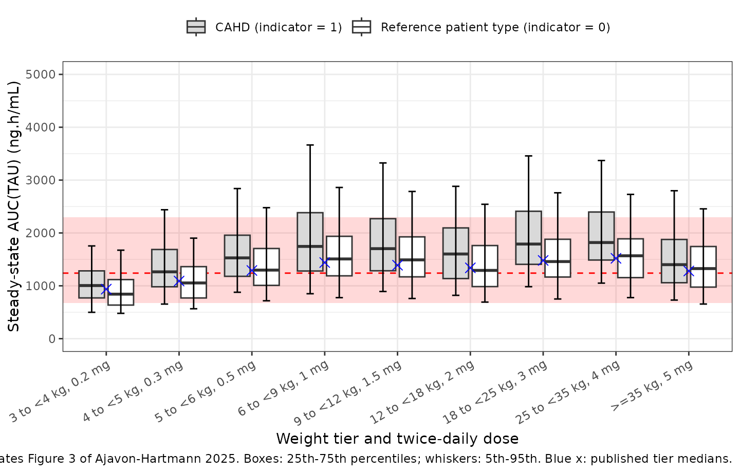
auc_med <- fig3_sim |>
  dplyr::group_by(tier, scenario) |>
  dplyr::summarise(sim = median(auc), .groups = "drop") |>
  tidyr::pivot_wider(names_from = scenario, values_from = sim) |>
  dplyr::inner_join(fig3_published, by = "tier") |>
  dplyr::mutate(
    pct_cahd = 100 * (`CAHD (indicator = 1)` / published - 1),
    pct_ref = 100 * (`Reference patient type (indicator = 0)` / published - 1)
  )
auc_med |>
  dplyr::rename(
    "Weight tier" = tier, "Figure 3 median" = published,
    "% difference, CAHD" = pct_cahd, "% difference, reference type" = pct_ref
  ) |>
knitr::kable(digits = 1, caption = "Steady-state AUC(TAU) medians (ng.h/mL) by simulated patient type.")| Weight tier | CAHD (indicator = 1) | Reference patient type (indicator = 0) | Figure 3 median | % difference, CAHD | % difference, reference type |
|---|---|---|---|---|---|
| 3 to <4 kg, 0.2 mg | 1005.0 | 842.2 | 937 | 7.3 | -10.1 |
| 4 to <5 kg, 0.3 mg | 1264.3 | 1054.1 | 1090 | 16.0 | -3.3 |
| 5 to <6 kg, 0.5 mg | 1528.2 | 1297.3 | 1290 | 18.5 | 0.6 |
| 6 to <9 kg, 1 mg | 1745.2 | 1508.3 | 1440 | 21.2 | 4.7 |
| 9 to <12 kg, 1.5 mg | 1703.0 | 1490.8 | 1390 | 22.5 | 7.2 |
| 12 to <18 kg, 2 mg | 1601.8 | 1291.6 | 1340 | 19.5 | -3.6 |
| 18 to <25 kg, 3 mg | 1790.0 | 1458.7 | 1480 | 20.9 | -1.4 |
| 25 to <35 kg, 4 mg | 1818.7 | 1568.2 | 1520 | 19.7 | 3.2 |
| >=35 kg, 5 mg | 1400.3 | 1325.8 | 1280 | 9.4 | 3.6 |
# A wrong clearance, weight exponent, maturation function, F1 or unit shifts
# every tier by tens of percent; the tier-to-tier spread reflects only how
# closely the CDC-based cohort reproduces the paper's age and weight sampling.
stopifnot(
  abs(median(auc_med$pct_ref)) < 10,
  all(abs(auc_med$pct_ref) < 25),
  # The CAHD scenario sits one CAHD effect, about 20%, above the figure.
  abs(median(auc_med$pct_cahd) - 100 * (exp(0.185) - 1)) < 10
)
Comparison against published values (Table 2)
Table 2 reports geometric means of the individual (Bayesian)
estimates for the 124 SAXOPHONE patients by weight tier.
ncaComparisonTable() compares the simulated medians of the
six SAXOPHONE tiers with them.
published <- tibble::tribble(
  ~tier,                  ~auclast, ~cmax, ~cmin, ~tmax,
  "6 to <9 kg, 1 mg",         1460,   185,  57.9,  2.14,
  "9 to <12 kg, 1.5 mg",      1840,   218,  82.7,  2.46,
  "12 to <18 kg, 2 mg",       1610,   222,  64.3,  1.72,
  "18 to <25 kg, 3 mg",       1760,   244,  67.4,  1.65,
  "25 to <35 kg, 4 mg",       1840,   249,  73.1,  1.69,
  ">=35 kg, 5 mg",            1630,   203,  72.7,  1.89
)

cmp <- nlmixr2lib::ncaComparisonTable(
  simulated = nca_res,
  reference = published,
  by = "tier",
  units = c(auclast = "ng.h/mL", cmax = "ng/mL", cmin = "ng/mL", tmax = "h"),
  tolerance_pct = 20
)
knitr::kable(
  cmp,
  caption = paste(
    "Simulated (median, virtual CAHD cohort) vs published (Table 2 geometric",
    "means of SAXOPHONE individual estimates). * differs from reference by >20%."
  )
)| NCA parameter | tier | Reference | Simulated | % diff |
|---|---|---|---|---|
| Cmax (ng/mL) | 6 to <9 kg, 1 mg | 185 | 194 | +5.1% |
| Cmax (ng/mL) | 9 to <12 kg, 1.5 mg | 218 | 227 | +4.2% |
| Cmax (ng/mL) | 12 to <18 kg, 2 mg | 222 | 212 | -4.3% |
| Cmax (ng/mL) | 18 to <25 kg, 3 mg | 244 | 243 | -0.6% |
| Cmax (ng/mL) | 25 to <35 kg, 4 mg | 249 | 238 | -4.5% |
| Cmax (ng/mL) | >=35 kg, 5 mg | 203 | 178 | -12.1% |
| Cmin (ng/mL) | 6 to <9 kg, 1 mg | 57.9 | 86.4 | +49.1%* |
| Cmin (ng/mL) | 9 to <12 kg, 1.5 mg | 82.7 | 69.3 | -16.2% |
| Cmin (ng/mL) | 12 to <18 kg, 2 mg | 64.3 | 64.9 | +1.0% |
| Cmin (ng/mL) | 18 to <25 kg, 3 mg | 67.4 | 77.8 | +15.4% |
| Cmin (ng/mL) | 25 to <35 kg, 4 mg | 73.1 | 83.6 | +14.3% |
| Cmin (ng/mL) | >=35 kg, 5 mg | 72.7 | 60.7 | -16.5% |
| Tmax (h) | 6 to <9 kg, 1 mg | 2.14 | 2.75 | +28.5%* |
| Tmax (h) | 9 to <12 kg, 1.5 mg | 2.46 | 1.75 | -28.9%* |
| Tmax (h) | 12 to <18 kg, 2 mg | 1.72 | 1.75 | +1.7% |
| Tmax (h) | 18 to <25 kg, 3 mg | 1.65 | 1.75 | +6.1% |
| Tmax (h) | 25 to <35 kg, 4 mg | 1.69 | 1.75 | +3.6% |
| Tmax (h) | >=35 kg, 5 mg | 1.89 | 1.75 | -7.4% |
| AUClast (ng.h/mL) | 6 to <9 kg, 1 mg | 1460 | 1750 | +19.5% |
| AUClast (ng.h/mL) | 9 to <12 kg, 1.5 mg | 1840 | 1700 | -7.4% |
| AUClast (ng.h/mL) | 12 to <18 kg, 2 mg | 1610 | 1600 | -0.5% |
| AUClast (ng.h/mL) | 18 to <25 kg, 3 mg | 1760 | 1790 | +1.7% |
| AUClast (ng.h/mL) | 25 to <35 kg, 4 mg | 1840 | 1820 | -1.2% |
| AUClast (ng.h/mL) | >=35 kg, 5 mg | 1630 | 1400 | -14.1% |
The two sides differ in kind: Table 2 summarises the empirical Bayes estimates of the actual SAXOPHONE patients, who had few samples each (shrinkage on the etas of ka, Q/F and Vp/F was 36 to 38%), while the simulation draws a full virtual cohort with the population variances. Only six patients sit in the 6 to <9 kg tier and two in the 9 to <12 kg tier, so those reference values are themselves imprecise. Cmax, Cmin and Tmax are therefore descriptive. AUC(TAU) is checked at the centre only: across the six tiers the median difference between the simulated CAHD medians and the Table 2 geometric means must be small.
t2_auc <- nca_wide |>
  dplyr::group_by(tier) |>
  dplyr::summarise(sim = median(auclast), .groups = "drop") |>
  dplyr::inner_join(published |> dplyr::select(tier, auclast), by = "tier") |>
  dplyr::mutate(pct_diff = 100 * (sim / auclast - 1))
stopifnot(nrow(t2_auc) == 6, abs(median(t2_auc$pct_diff)) < 10)
Figure 4: anti-factor Xa activity
The PK/PD model is a zero-intercept line with a normally distributed slope (mean 0.916, SD 0.0528) and an additive residual SD of 12.8 ng/mL. The simulated AXA below is computed from the model-predicted concentration, so the scatter about the line combines the slope variability and the residual error. Figure 4 plots observed AXA against observed apixaban concentration.
ini_df <- rxode2::rxode2(mod)$iniDf
#> ℹ parameter labels from comments will be replaced by 'label()'
stopifnot(
  abs(ini_df$est[ini_df$name == "slope_antiFXa"] - 0.916) < 1e-9,
  abs(sqrt(ini_df$est[ini_df$name == "etaslope_antiFXa"]) - 0.0528) < 1e-6
)

# Add the residual error to the PK/PD output: rxSolve returns predictions
# without residual error for each endpoint.
set.seed(20250624)
axa_obs <- sim_nca |>
  dplyr::slice_sample(n = 3000) |>
  dplyr::mutate(antiFXa_obs = antiFXa + stats::rnorm(dplyr::n(), 0, 12.8))

ggplot(axa_obs, aes(Cc, antiFXa_obs)) +
  geom_point(alpha = 0.15, size = 0.6) +
  geom_abline(slope = 0.916, intercept = 0) +
  labs(
    x = "Apixaban concentration (ng/mL)", y = "Anti-FXa activity (ng/mL)",
    caption = "Model relationship underlying Figure 4 of Ajavon-Hartmann 2025 (median line)."
  ) +
  theme_bw()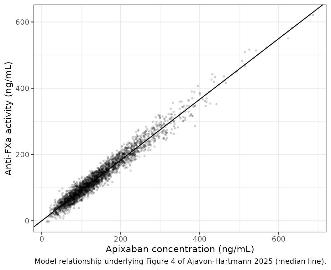
# The ratio antiFXa / Cc is each patient's slope, so its distribution must
# reproduce the Table 3 mean and SD.
slopes <- sim |>
  dplyr::filter(Cc > 1) |>
  dplyr::distinct(id, .keep_all = TRUE) |>
  dplyr::mutate(slope = antiFXa / Cc)
stopifnot(
  abs(mean(slopes$slope) - 0.916) < 0.01,
  abs(stats::sd(slopes$slope) - 0.0528) < 0.01
)
Assumptions and deviations
- Figure 3 patient type. The Methods describe the Figure 3 virtual patients as children with CAHD, but the published tier medians are reproduced only when the CAHD effect on CL/F is switched off, and sit about 20% (exp(0.185)) below the CAHD simulation and below the Table 2 AUC(TAU) of the real SAXOPHONE patients. The model keeps the published CAHD effect; the vignette shows both simulated patient types and gates Figure 3 against the reference-type scenario.
-
Patient-type covariates. The paper’s single
patient-type variable (
PTYPE) is carried as two binary indicators.DIS_ALL= 1 for the PREVAPIX-ALL patients (acute lymphoblastic leukemia or lymphoblastic lymphoma on asparaginase, pooled as in the paper’s footnote) andDIS_HEART_CONGENITAL_ACQUIRED= 1 for the SAXOPHONE patients; both 0 selects healthy adults and the pediatric phase I patients at risk of thromboembolism. The ALL/LL indicator acts on ka only, the CAHD indicator on CL/F only. The authors suggest the lower CL/F in CAHD reflects the Fontan circulation of most SAXOPHONE patients; the indicator is also confounded with study. -
PED9M is derived inside the model from
AGE(1 for 9 months <= age <18 years), matching the Table 1 footnote definition. -
Formulation. The sprinkle-capsule relative
bioavailability (1.1, fixed) is carried by the general capsule indicator
FORM_CAPSULE(1 = sprinkle capsule); the reference is tablet or oral solution. The paper does not say which SAXOPHONE patients took the sprinkle capsule, so all virtual patients here take the reference formulation. -
Dose-dependent bioavailability reads the dose from
the
DOSE_APIXABAN_MGcolumn, which must equal the event-tableamton the dose records. The SAXOPHONE doses per weight tier are not tabulated; the doses used are the regimen proposed in the Results, which the Table 2 consistency check above confirms. -
PK/PD random effect. Table 3 reports a
random-effect standard deviation of 0.0528 for the linear mixed-effects
regression with ‘IIV in the slope parameter’ (Discussion). It is encoded
as a normally distributed, additive random effect on the slope
(
slope_antiFXa + etaslope_antiFXa), the usual form of a linear mixed-effects random slope. The PK/PD model was fitted to observed apixaban concentrations; here it is driven by the model-predicted concentrationCc. - PK/PD dataset size. The Methods give 541 concentrations from 253 patients for the PK/PD dataset; the Results give 390 AXA values from 123 patients after excluding values below the 35 ng/mL quantification limit and values without a time-matched concentration. The model metadata quotes the Results.
- Virtual cohort. Weight-for-age uses the CDC 2000 sex-averaged median with 12% lognormal scatter instead of sampling the full sex-specific distribution, and ages are drawn within each weight tier. This mainly affects the age and weight mix inside a tier, and so the tier medians, by a few percent. The three lightest tiers (3 to <6 kg) are below the weight of any SAXOPHONE patient and are model extrapolations, as in the paper.
- Cohort size. 200 virtual patients per tier, against the paper’s about 1000 per tier.
- Adult reference. The adult VTE-treatment median of 1240 ng.h/mL (90% CI 675-2300) is taken from the paper’s text; adults are not simulated here.
- No erratum or correction notice for this article was found as of 2026-11-10.