Paracetamol and its metabolites in spinal muscular atrophy (Zhao 2025)
Source:vignettes/articles/Zhao_2025_paracetamol.Rmd
Zhao_2025_paracetamol.RmdModel and source
mod_meta <- nlmixr2est::nlmixr(readModelDb("Zhao_2025_paracetamol"))$meta
#> ℹ parameter labels from comments will be replaced by 'label()'- Citation: Zhao Q, Naume MM, de Winter BCM, Krag T, Haslund-Krog SS, Revsbech KL, Vissing J, Holst H, Moller MH, Hornsyld TM, Duno M, Hoei-Hansen CE, Born AP, Jensen PB, Orngreen MC (2025). Paracetamol and its metabolites in children and adults with spinal muscular atrophy - a population pharmacokinetic model. Br J Clin Pharmacol 91(7):2045-2056. doi:10.1002/bcp.70028.
- Article: https://doi.org/10.1002/bcp.70028
- Description: Parent-and-metabolites population PK model for oral paracetamol and its glucuronide, sulphate and combined oxidative (cysteine + mercapturate) metabolites in children and adults with spinal muscular atrophy (SMA) and healthy controls (Zhao 2025). One compartment per compound with first-order absorption through a depot, a fixed absorption lag time, and body-weight allometric scaling (exponent fixed at 0.75 on every clearance and 1 on every volume). Paracetamol leaves the central compartment by four parallel first-order routes: glucuronide formation, sulphate formation, oxidative-metabolite formation, and a leftover clearance covering unchanged drug plus any unaccounted route. Each metabolite has its own one-compartment plasma pool with an apparent volume fixed at 18% of the paracetamol volume and its own first-order elimination clearance. SMA disease status raises the paracetamol volume of distribution (and, through the fixed 0.18 ratio, every metabolite volume) by 58%; plasma myoglobin scales the paracetamol leftover clearance with a negative power exponent, and plasma total bilirubin scales sulphate-formation clearance positively and oxidative-metabolite elimination clearance negatively.
Population
Zhao et al. (2025) analysed a Danish single-centre trial (EudraCT 2018-002295-40) in which six adults with spinal muscular atrophy (SMA), six children with SMA and 11 healthy controls received oral paracetamol 15 mg/kg every 6 h for three days, capped at a maximum single dose of 1 g (Methods section 2.1). Blood was sampled hourly for 6-8 h on Days 1 and 3 after a pre-treatment baseline sample, giving 294 plasma samples per analyte for each of paracetamol, paracetamol-glucuronide, paracetamol-sulphate and the combined oxidative metabolites (cysteine conjugate + mercapturic acid).
The two groups differ sharply in size and in the two retained biochemical covariates (Table 1 of the source): median body weight 30.5 kg (range 22-57) in SMA versus 78.0 kg (51-103) in healthy controls; median plasma myoglobin 17 ng/mL (14-54) versus 34 ng/mL (17-74); median total bilirubin 4 umol/L (2-25) versus 7 umol/L (3-15). Median age was 17 years (6-37) in the SMA group and 25 years (20-36) in the controls; 10 of 23 participants (43.5%) were female.
The same information is available programmatically via
readModelDb("Zhao_2025_paracetamol")$population.
Source trace
Every ini() entry in
inst/modeldb/specificDrugs/Zhao_2025_paracetamol.R carries
an in-file comment naming its source location. The table below collects
them for review.
| Component | Value | Source location |
|---|---|---|
| Structural model | 1 cmt per compound, first-order absorption + lag, allometric WT | Figure 1 (schematic) and Results section 3.2 |
| Covariate model form | Eq. 1 (categorical, proportional) and Eq. 2 (continuous, median-normalised power) | Supplementary material 1, Methods for model building |
| t_lag | 0.153 h (FIX) | Table 2, row ‘t lag (h) (FIX)’ + table footnote |
| k_a | 2.84 1/h | Table 2, final model column |
| V_pcm/F | 63.5 L/70 kg | Table 2, final model column |
| CL_p/F (leftover) | 8.16 L/h/70 kg | Table 2, final model column |
| CL_pg/F (glucuronide formation) | 6.37 L/h/70 kg | Table 2, final model column |
| CL_ps/F (sulphate formation) | 8.43 L/h/70 kg | Table 2, final model column |
| CL_pox/F (oxidative formation) | 0.20 L/h/70 kg | Table 2, final model column |
| CL_gluc/F (glucuronide elimination) | 5.69 L/h/70 kg | Table 2, final model column |
| CL_sulf/F (sulphate elimination) | 20.4 L/h/70 kg | Table 2, final model column |
| CL_ox/F (oxidative elimination) | 3.72 L/h/70 kg | Table 2, final model column |
| Metabolite volumes | 0.18 * V_pcm/F = 11.43 L/70 kg | Methods section 2.2 and Table 2 rows V_glu/V_sulf/V_ox |
| Allometric exponents | 0.75 on CL, 1 on V (both FIX) | Table 2 caption and Results section 3.2 |
| Disease effect on V_pcm/F | 1.58 | Table 2, ‘Covariate effect on V_pcm/F – Disease’ |
| Myoglobin on CL_p/F | -1.10 (per MYO/25) | Table 2 + Results section 3.3 (‘negative correlation’) |
| Bilirubin on CL_ps/F | +0.18 (per TBILI/6) | Table 2 + Results section 3.3 (‘positive correlation’) |
| Bilirubin on CL_ox/F | -0.177 (per TBILI/6) | Table 2 + Results section 3.3 (‘negative correlation’) |
| BSV (all six etas) | omega (log-SD) x 100, per Table 2 ‘BSV (%)’ | Table 2 + Discussion (CL_p/F CV 105% = sqrt(exp(0.862^2) - 1)) |
| Proportional residual error | 0.28 / 0.18 / 0.22 / 0.17 | Table 2, ‘Residual variability – Proportional’ |
Two values whose sign the typeset table loses
Table 2 prints the myoglobin exponent as 1.10 and the
bilirubin-on-CL_ox exponent as 0.177, but their bootstrap
confidence intervals are printed in descending order
(3.07 - 0.49 and 0.45 - 0.03), which is only
possible for negative intervals, and Results section 3.3 states both
correlations are negative. The signs are confirmed numerically by
supplementary Table S3: the paracetamol half-life rises monotonically
with myoglobin (2.20 h at 15 ng/mL to 3.69 h at 70 ng/mL, i.e. clearance
falls), and the oxidative-metabolite half-life rises monotonically with
bilirubin (3.18 h at 3 umol/L to 4.19 h at 24 umol/L). Both exponents
are therefore encoded as negative.
Concentration scale: molar, not paracetamol-mass
Zhao 2025 never states the amount scale of its metabolite compartments, and the choice is load-bearing: paracetamol converts 1:1 on a molar basis to each conjugate, so a parent-metabolite model with a single set of formation and elimination clearances is only self-consistent when the compartments carry moles. The paper’s own simulation output settles it, because the steady-state exposure ratio of a metabolite to the parent is volume-independent – it equals CL_formation / CL_elimination in whatever amount unit the compartments carry, so it discriminates the amount scale without depending on any volume. Reproducing the model on the molar scale and converting each output to that species’ own mass units matches supplementary Table S2 to within 2.5%; a paracetamol-mass parameterisation is 34-53% low. The check is run on the simulated 0-24 h window (the same window Table S2 reports) in the “Structural identity” section below.
Virtual cohort
The published simulations (Figures 2-4 and supplementary Tables S2 and S3) all use SMA patients dosed 15 mg/kg every 6 h (capped at 1 g), varying one covariate at a time and holding the others at the population median (myoglobin 25 ng/mL, total bilirubin 6 umol/L – the same medians Table 2 uses to normalise the two power models). Twelve typical-value scenarios reproduce the three published simulation panels.
mw <- c(pcm = 151.16, gluc = 327.29, sulf = 231.23, cysmer = 270.30)

scenarios <- dplyr::bind_rows(
  tibble::tibble(panel = "Body weight (Table S2)",
                 WT = c(70, 50, 35, 27), MYO = 25, TBILI = 6),
  tibble::tibble(panel = "Myoglobin (Table S3)",
                 WT = 70, MYO = c(15, 25, 40, 70), TBILI = 6),
  tibble::tibble(panel = "Bilirubin (Table S3)",
                 WT = 70, MYO = 25, TBILI = c(3, 6, 12, 24))
) |>
  dplyr::mutate(
    DIS_HEALTHY = 0,
    id        = dplyr::row_number(),
    dose_mg   = pmin(1000, 15 * WT),
    dose_umol = dose_mg / mw[["pcm"]] * 1000,
    scenario  = dplyr::case_when(
      panel == "Body weight (Table S2)" ~ paste0("WT ", WT, " kg"),
      panel == "Myoglobin (Table S3)"   ~ paste0("MYO ", MYO, " ng/mL"),
      TRUE                              ~ paste0("BILI ", TBILI, " umol/L")
    )
  )

knitr::kable(
  scenarios |> dplyr::select(panel, scenario, WT, MYO, TBILI, dose_mg, dose_umol),
  digits = 1,
  caption = "Twelve typical-value SMA scenarios reproducing the published simulations."
)| panel | scenario | WT | MYO | TBILI | dose_mg | dose_umol |
|---|---|---|---|---|---|---|
| Body weight (Table S2) | WT 70 kg | 70 | 25 | 6 | 1000 | 6615.5 |
| Body weight (Table S2) | WT 50 kg | 50 | 25 | 6 | 750 | 4961.6 |
| Body weight (Table S2) | WT 35 kg | 35 | 25 | 6 | 525 | 3473.1 |
| Body weight (Table S2) | WT 27 kg | 27 | 25 | 6 | 405 | 2679.3 |
| Myoglobin (Table S3) | MYO 15 ng/mL | 70 | 15 | 6 | 1000 | 6615.5 |
| Myoglobin (Table S3) | MYO 25 ng/mL | 70 | 25 | 6 | 1000 | 6615.5 |
| Myoglobin (Table S3) | MYO 40 ng/mL | 70 | 40 | 6 | 1000 | 6615.5 |
| Myoglobin (Table S3) | MYO 70 ng/mL | 70 | 70 | 6 | 1000 | 6615.5 |
| Bilirubin (Table S3) | BILI 3 umol/L | 70 | 25 | 3 | 1000 | 6615.5 |
| Bilirubin (Table S3) | BILI 6 umol/L | 70 | 25 | 6 | 1000 | 6615.5 |
| Bilirubin (Table S3) | BILI 12 umol/L | 70 | 25 | 12 | 1000 | 6615.5 |
| Bilirubin (Table S3) | BILI 24 umol/L | 70 | 25 | 24 | 1000 | 6615.5 |
obs_times <- seq(0, 24, by = 0.1)

doses <- scenarios |>
  tidyr::expand_grid(time = c(0, 6, 12, 18)) |>
  dplyr::mutate(cmt = "depot", amt = dose_umol, evid = 1L) |>
  dplyr::select(id, time, cmt, amt, evid, WT, MYO, TBILI, DIS_HEALTHY)

obs <- scenarios |>
  dplyr::select(id, WT, MYO, TBILI, DIS_HEALTHY) |>
  tidyr::expand_grid(time = obs_times) |>
  dplyr::mutate(cmt = "Cc", amt = NA_real_, evid = 0L) |>
  dplyr::select(id, time, cmt, amt, evid, WT, MYO, TBILI, DIS_HEALTHY)

events <- dplyr::bind_rows(doses, obs) |>
  dplyr::arrange(id, time, dplyr::desc(evid))
Simulation
Typical-value trajectories use rxode2::zeroRe() so that
the comparison against the published typical simulations is not blurred
by the (very large) between-subject variability on k_a and
CL_p/F.
mod <- readModelDb("Zhao_2025_paracetamol")
mod_typ <- rxode2::zeroRe(mod)
#> ℹ parameter labels from comments will be replaced by 'label()'

sim <- rxode2::rxSolve(mod_typ, events = events, omega = NA, sigma = NA) |>
  as.data.frame() |>
  dplyr::left_join(dplyr::select(scenarios, id, panel, scenario), by = "id")

stopifnot(dplyr::n_distinct(sim$id) == nrow(scenarios))

# Convert each analyte from umol/L to its own mass concentration (ug/L),
# which is the scale the published figures and supplementary tables use.
sim <- sim |>
  dplyr::mutate(
    pcm_ugL    = Cc        * mw[["pcm"]],
    gluc_ugL   = Cc_gluc   * mw[["gluc"]],
    sulf_ugL   = Cc_sulf   * mw[["sulf"]],
    cysmer_ugL = Cc_cysmer * mw[["cysmer"]]
  )
Replicate Figure 2 – body-weight effect in SMA patients
long_ugL <- function(d) {
  d |>
    tidyr::pivot_longer(
      c(pcm_ugL, gluc_ugL, sulf_ugL, cysmer_ugL),
      names_to = "analyte", values_to = "conc"
    ) |>
    dplyr::mutate(analyte = factor(
      analyte,
      levels = c("pcm_ugL", "gluc_ugL", "sulf_ugL", "cysmer_ugL"),
      labels = c("(A) Paracetamol", "(B) Glucuronide",
                 "(C) Sulphate", "(D) Oxidative metabolites")
    ))
}

sim |>
  dplyr::filter(panel == "Body weight (Table S2)") |>
  long_ugL() |>
  ggplot(aes(time, conc, colour = scenario)) +
  geom_line() +
  facet_wrap(~analyte, scales = "free_y") +
  labs(x = "Time (h)", y = "Concentration (ug/L)", colour = "Scenario",
       title = "Body-weight effect in SMA patients (15 mg/kg q6h, capped at 1 g)",
       caption = "Replicates Figure 2 of Zhao 2025.") +
  theme_minimal()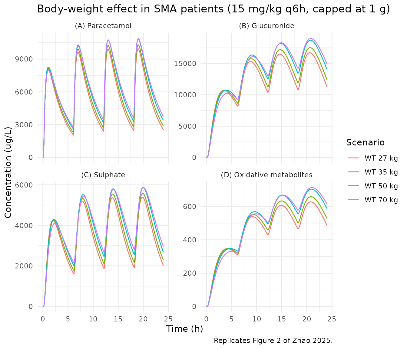
Replicate Figure 3 – myoglobin effect in 70 kg SMA patients
sim |>
  dplyr::filter(panel == "Myoglobin (Table S3)") |>
  long_ugL() |>
  ggplot(aes(time, conc, colour = scenario)) +
  geom_line() +
  facet_wrap(~analyte, scales = "free_y") +
  labs(x = "Time (h)", y = "Concentration (ug/L)", colour = "Myoglobin",
       title = "Myoglobin effect in 70 kg SMA patients (1000 mg q6h)",
       caption = "Replicates Figure 3 of Zhao 2025.") +
  theme_minimal()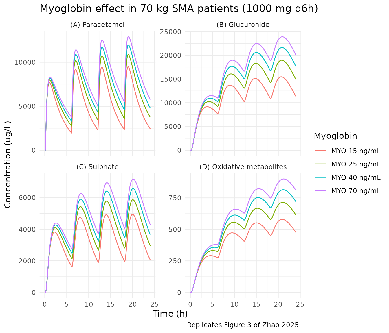
Replicate Figure 4 – bilirubin effect in 70 kg SMA patients
sim |>
  dplyr::filter(panel == "Bilirubin (Table S3)") |>
  long_ugL() |>
  ggplot(aes(time, conc, colour = scenario)) +
  geom_line() +
  facet_wrap(~analyte, scales = "free_y") +
  labs(x = "Time (h)", y = "Concentration (ug/L)", colour = "Bilirubin",
       title = "Bilirubin effect in 70 kg SMA patients (1000 mg q6h)",
       caption = "Replicates Figure 4 of Zhao 2025.") +
  theme_minimal()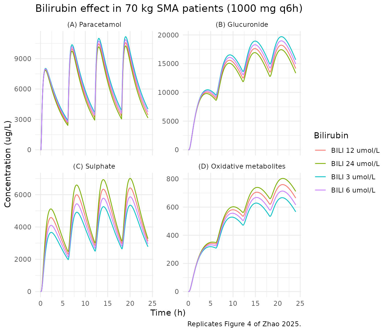
The absolute levels are the first check on the molar reading: at myoglobin 25 ng/mL and bilirubin 6 umol/L the simulated 70 kg SMA patient sits at roughly 3000-11000 ug/L paracetamol, 11000-18000 ug/L glucuronide, 2500-6000 ug/L sulphate and 400-700 ug/L oxidative metabolites, matching the axis ranges of Figures 2-4 of the source.
PKNCA validation
nca_one <- function(conc_col) {
  cdat <- sim |>
    dplyr::select(id, time, scenario, conc = dplyr::all_of(conc_col)) |>
    dplyr::filter(!is.na(conc))
  ddat <- scenarios |>
    dplyr::select(id, scenario, amt = dose_umol) |>
    tidyr::expand_grid(time = c(0, 6, 12, 18))
  obj <- PKNCA::PKNCAdata(
    PKNCA::PKNCAconc(cdat, conc ~ time | scenario + id),
    PKNCA::PKNCAdose(ddat, amt ~ time | scenario + id),
    intervals = data.frame(
      start = 0, end = 24,
      cmax = TRUE, tmax = TRUE, auclast = TRUE, half.life = TRUE
    )
  )
  as.data.frame(PKNCA::pk.nca(obj)$result) |>
    dplyr::mutate(analyte = conc_col)
}

nca <- dplyr::bind_rows(lapply(
  c("pcm_ugL", "gluc_ugL", "sulf_ugL", "cysmer_ugL"), nca_one
))

nca_wide <- nca |>
  dplyr::select(scenario, analyte, PPTESTCD, PPORRES) |>
  tidyr::pivot_wider(names_from = PPTESTCD, values_from = PPORRES)

knitr::kable(
  nca_wide |>
    dplyr::rename("Scenario" = scenario, "Analyte" = analyte,
                  "Cmax (ug/L)" = cmax, "Tmax (h)" = tmax,
                  "AUC0-24 (ug*h/L)" = auclast, "t1/2 (h)" = half.life),
  digits = c(0, 0, 0, 2, 0, 2),
  caption = paste(
    "Simulated typical-value NCA over 0-24 h for all four analytes.",
    "Half-life is the NCA terminal half-life from the simulated profile,",
    "which for a metabolite is formation-rate limited and therefore tracks",
    "the parent -- it is not comparable to the V/CL half-lives the paper",
    "tabulates (see below)."
  )
)| Scenario | Analyte | AUC0-24 (ug*h/L) | Cmax (ug/L) | Tmax (h) | tlast | lambda.z | r.squared | adj.r.squared | lambda.z.time.first | lambda.z.time.last | lambda.z.n.points | clast.pred | t1/2 (h) | span.ratio |
|---|---|---|---|---|---|---|---|---|---|---|---|---|---|---|
| BILI 12 umol/L | pcm_ugL | 150547 | 10571.41 | 19 | 24 | 0 | 1 | 1 | 19.6 | 24 | 45 | 3454 | 3 | 2 |
| BILI 24 umol/L | pcm_ugL | 144240 | 10257.26 | 19 | 24 | 0 | 1 | 1 | 19.6 | 24 | 45 | 3156 | 3 | 2 |
| BILI 3 umol/L | pcm_ugL | 162254 | 11168.33 | 19 | 24 | 0 | 1 | 1 | 19.6 | 24 | 45 | 4032 | 3 | 1 |
| BILI 6 umol/L | pcm_ugL | 156560 | 10875.78 | 19 | 24 | 0 | 1 | 1 | 19.6 | 24 | 45 | 3747 | 3 | 1 |
| MYO 15 ng/mL | pcm_ugL | 128174 | 9480.54 | 19 | 24 | 0 | 1 | 1 | 19.6 | 24 | 45 | 2440 | 2 | 2 |
| MYO 25 ng/mL | pcm_ugL | 156560 | 10875.78 | 19 | 24 | 0 | 1 | 1 | 19.6 | 24 | 45 | 3747 | 3 | 1 |
| MYO 40 ng/mL | pcm_ugL | 177148 | 11953.20 | 19 | 24 | 0 | 1 | 1 | 19.6 | 24 | 45 | 4811 | 4 | 1 |
| MYO 70 ng/mL | pcm_ugL | 194212 | 12885.75 | 19 | 24 | 0 | 1 | 1 | 19.7 | 24 | 44 | 5759 | 4 | 1 |
| WT 27 kg | pcm_ugL | 134281 | 9940.32 | 19 | 24 | 0 | 1 | 1 | 19.6 | 24 | 45 | 2549 | 2 | 2 |
| WT 35 kg | pcm_ugL | 142052 | 10311.30 | 19 | 24 | 0 | 1 | 1 | 19.6 | 24 | 45 | 2886 | 3 | 2 |
| WT 50 kg | pcm_ugL | 153261 | 10859.66 | 19 | 24 | 0 | 1 | 1 | 19.6 | 24 | 45 | 3398 | 3 | 2 |
| WT 70 kg | pcm_ugL | 156560 | 10875.78 | 19 | 24 | 0 | 1 | 1 | 19.6 | 24 | 45 | 3747 | 3 | 1 |
| BILI 12 umol/L | gluc_ugL | 319898 | 18211.47 | 21 | 24 | 0 | 1 | 1 | 23.7 | 24 | 4 | 14154 | 6 | 0 |
| BILI 24 umol/L | gluc_ugL | 307153 | 17424.57 | 21 | 24 | 0 | 1 | 1 | 23.6 | 24 | 5 | 13355 | 5 | 0 |
| BILI 3 umol/L | gluc_ugL | 343444 | 19694.72 | 21 | 24 | 0 | 1 | 1 | 23.7 | 24 | 4 | 15675 | 6 | 0 |
| BILI 6 umol/L | gluc_ugL | 332011 | 18969.70 | 21 | 24 | 0 | 1 | 1 | 23.7 | 24 | 4 | 14930 | 6 | 0 |
| MYO 15 ng/mL | gluc_ugL | 274493 | 15466.49 | 21 | 24 | 0 | 1 | 1 | 23.6 | 24 | 5 | 11375 | 5 | 0 |
| MYO 25 ng/mL | gluc_ugL | 332011 | 18969.70 | 21 | 24 | 0 | 1 | 1 | 23.7 | 24 | 4 | 14930 | 6 | 0 |
| MYO 40 ng/mL | gluc_ugL | 373197 | 21625.63 | 21 | 24 | 0 | 1 | 1 | 23.7 | 24 | 4 | 17676 | 7 | 0 |
| MYO 70 ng/mL | gluc_ugL | 407006 | 23897.51 | 21 | 24 | 0 | 1 | 1 | 23.7 | 24 | 4 | 20055 | 7 | 0 |
| WT 27 kg | gluc_ugL | 297084 | 16721.08 | 21 | 24 | 0 | 1 | 1 | 23.6 | 24 | 5 | 11317 | 4 | 0 |
| WT 35 kg | gluc_ugL | 311039 | 17517.75 | 21 | 24 | 0 | 1 | 1 | 23.6 | 24 | 5 | 12435 | 4 | 0 |
| WT 50 kg | gluc_ugL | 330380 | 18706.37 | 21 | 24 | 0 | 1 | 1 | 23.6 | 24 | 5 | 14058 | 5 | 0 |
| WT 70 kg | gluc_ugL | 332011 | 18969.70 | 21 | 24 | 0 | 1 | 1 | 23.7 | 24 | 4 | 14930 | 6 | 0 |
| BILI 12 umol/L | sulf_ugL | 105017 | 6419.65 | 20 | 24 | 0 | 1 | 1 | 22.5 | 24 | 16 | 3125 | 3 | 0 |
| BILI 24 umol/L | sulf_ugL | 114086 | 7006.98 | 20 | 24 | 0 | 1 | 1 | 22.5 | 24 | 16 | 3279 | 3 | 1 |
| BILI 3 umol/L | sulf_ugL | 88053 | 5347.82 | 20 | 24 | 0 | 1 | 1 | 22.5 | 24 | 16 | 2779 | 3 | 0 |
| BILI 6 umol/L | sulf_ugL | 96324 | 5866.68 | 20 | 24 | 0 | 1 | 1 | 22.5 | 24 | 16 | 2957 | 3 | 0 |
| MYO 15 ng/mL | sulf_ugL | 79175 | 4944.55 | 20 | 24 | 0 | 1 | 1 | 22.5 | 24 | 16 | 2059 | 3 | 1 |
| MYO 25 ng/mL | sulf_ugL | 96324 | 5866.68 | 20 | 24 | 0 | 1 | 1 | 22.5 | 24 | 16 | 2957 | 3 | 0 |
| MYO 40 ng/mL | sulf_ugL | 108709 | 6574.34 | 20 | 24 | 0 | 1 | 1 | 22.5 | 24 | 16 | 3667 | 4 | 0 |
| MYO 70 ng/mL | sulf_ugL | 118942 | 7184.46 | 20 | 24 | 0 | 1 | 1 | 22.5 | 24 | 16 | 4293 | 4 | 0 |
| WT 27 kg | sulf_ugL | 83447 | 5395.12 | 20 | 24 | 0 | 1 | 1 | 21.9 | 24 | 22 | 2021 | 2 | 1 |
| WT 35 kg | sulf_ugL | 88067 | 5583.52 | 20 | 24 | 0 | 1 | 1 | 22.1 | 24 | 20 | 2286 | 3 | 1 |
| WT 50 kg | sulf_ugL | 94668 | 5865.53 | 20 | 24 | 0 | 1 | 1 | 22.3 | 24 | 18 | 2687 | 3 | 1 |
| WT 70 kg | sulf_ugL | 96324 | 5866.68 | 20 | 24 | 0 | 1 | 1 | 22.5 | 24 | 16 | 2957 | 3 | 0 |
| BILI 12 umol/L | cysmer_ugL | 12714 | 759.86 | 21 | 24 | 0 | 1 | 1 | 23.7 | 24 | 4 | 664 | 9 | 0 |
| BILI 24 umol/L | cysmer_ugL | 13305 | 803.73 | 21 | 24 | 0 | 1 | 1 | 23.7 | 24 | 4 | 711 | 10 | 0 |
| BILI 3 umol/L | cysmer_ugL | 11362 | 666.81 | 21 | 24 | 0 | 1 | 1 | 23.7 | 24 | 4 | 566 | 8 | 0 |
| BILI 6 umol/L | cysmer_ugL | 12060 | 713.83 | 21 | 24 | 0 | 1 | 1 | 23.7 | 24 | 4 | 615 | 8 | 0 |
| MYO 15 ng/mL | cysmer_ugL | 10001 | 579.97 | 21 | 24 | 0 | 1 | 1 | 23.7 | 24 | 4 | 477 | 7 | 0 |
| MYO 25 ng/mL | cysmer_ugL | 12060 | 713.83 | 21 | 24 | 0 | 1 | 1 | 23.7 | 24 | 4 | 615 | 8 | 0 |
| MYO 40 ng/mL | cysmer_ugL | 13527 | 814.61 | 21 | 24 | 0 | 1 | 1 | 23.7 | 24 | 4 | 721 | 10 | 0 |
| MYO 70 ng/mL | cysmer_ugL | 14728 | 900.38 | 21 | 24 | 0 | 1 | 1 | 23.7 | 24 | 4 | 812 | 11 | 0 |
| WT 27 kg | cysmer_ugL | 11043 | 627.58 | 21 | 24 | 0 | 1 | 1 | 23.7 | 24 | 4 | 487 | 5 | 0 |
| WT 35 kg | cysmer_ugL | 11495 | 658.96 | 21 | 24 | 0 | 1 | 1 | 23.7 | 24 | 4 | 528 | 6 | 0 |
| WT 50 kg | cysmer_ugL | 12107 | 704.50 | 21 | 24 | 0 | 1 | 1 | 23.7 | 24 | 4 | 588 | 7 | 0 |
| WT 70 kg | cysmer_ugL | 12060 | 713.83 | 21 | 24 | 0 | 1 | 1 | 23.7 | 24 | 4 | 615 | 8 | 0 |
Comparison against the published AUC(0-24 h)
Supplementary Tables S2 and S3 report the median AUC(0-24 h) of 1000
simulated subjects for each scenario. The comparison below is against
the typical-value (zero-variability) trajectory, so a small systematic
offset is expected: with the very skewed between-subject distribution on
CL_p/F (omega = 0.862), the median of the individual total
clearances exceeds the typical value, so the published medians sit
slightly below the typical-value AUC.
ref_auc <- tibble::tribble(
  ~scenario,           ~pcm_ugL, ~gluc_ugL, ~sulf_ugL, ~cysmer_ugL,
  "WT 70 kg",            147330,    304768,     89652,       11152,
  "WT 50 kg",            143339,    298104,     88688,       11294,
  "WT 35 kg",            133833,    289267,     84298,       11141,
  "WT 27 kg",            123959,    263171,     76024,        9898,
  "MYO 15 ng/mL",        121164,    252827,     74728,        9197,
  "MYO 25 ng/mL",        146178,    301519,     89376,       11242,
  "MYO 40 ng/mL",        166944,    346387,    103558,       12789,
  "MYO 70 ng/mL",        178697,    366287,    109699,       13186,
  "BILI 3 umol/L",       152463,    315236,     81747,       10538,
  "BILI 6 umol/L",       146178,    301519,     89376,       11242,
  "BILI 12 umol/L",      141846,    298449,    100237,       12155,
  "BILI 24 umol/L",      131999,    271035,    104188,       11841
) |>
  tidyr::pivot_longer(-scenario, names_to = "analyte", values_to = "auclast")

auc_cmp <- nca_wide |>
  dplyr::select(scenario, analyte, simulated = auclast) |>
  dplyr::inner_join(ref_auc, by = c("scenario", "analyte")) |>
  dplyr::mutate(
    analyte = dplyr::recode(analyte,
      pcm_ugL = "Paracetamol", gluc_ugL = "Glucuronide",
      sulf_ugL = "Sulphate", cysmer_ugL = "Oxidative"),
    "% diff" = round(100 * (simulated - auclast) / auclast, 1)
  ) |>
  dplyr::rename("Scenario" = scenario, "Analyte" = analyte,
                "Published (ug*h/L)" = auclast,
                "Simulated (ug*h/L)" = simulated)

knitr::kable(auc_cmp, digits = 0,
caption = "AUC(0-24 h): simulated typical value vs published median of 1000 subjects (supplementary Tables S2 and S3).")| Scenario | Analyte | Simulated (ug*h/L) | Published (ug*h/L) | % diff |
|---|---|---|---|---|
| BILI 12 umol/L | Paracetamol | 150547 | 141846 | 6 |
| BILI 24 umol/L | Paracetamol | 144240 | 131999 | 9 |
| BILI 3 umol/L | Paracetamol | 162254 | 152463 | 6 |
| BILI 6 umol/L | Paracetamol | 156560 | 146178 | 7 |
| MYO 15 ng/mL | Paracetamol | 128174 | 121164 | 6 |
| MYO 25 ng/mL | Paracetamol | 156560 | 146178 | 7 |
| MYO 40 ng/mL | Paracetamol | 177148 | 166944 | 6 |
| MYO 70 ng/mL | Paracetamol | 194212 | 178697 | 9 |
| WT 27 kg | Paracetamol | 134281 | 123959 | 8 |
| WT 35 kg | Paracetamol | 142052 | 133833 | 6 |
| WT 50 kg | Paracetamol | 153261 | 143339 | 7 |
| WT 70 kg | Paracetamol | 156560 | 147330 | 6 |
| BILI 12 umol/L | Glucuronide | 319898 | 298449 | 7 |
| BILI 24 umol/L | Glucuronide | 307153 | 271035 | 13 |
| BILI 3 umol/L | Glucuronide | 343444 | 315236 | 9 |
| BILI 6 umol/L | Glucuronide | 332011 | 301519 | 10 |
| MYO 15 ng/mL | Glucuronide | 274493 | 252827 | 9 |
| MYO 25 ng/mL | Glucuronide | 332011 | 301519 | 10 |
| MYO 40 ng/mL | Glucuronide | 373197 | 346387 | 8 |
| MYO 70 ng/mL | Glucuronide | 407006 | 366287 | 11 |
| WT 27 kg | Glucuronide | 297084 | 263171 | 13 |
| WT 35 kg | Glucuronide | 311039 | 289267 | 8 |
| WT 50 kg | Glucuronide | 330380 | 298104 | 11 |
| WT 70 kg | Glucuronide | 332011 | 304768 | 9 |
| BILI 12 umol/L | Sulphate | 105017 | 100237 | 5 |
| BILI 24 umol/L | Sulphate | 114086 | 104188 | 10 |
| BILI 3 umol/L | Sulphate | 88053 | 81747 | 8 |
| BILI 6 umol/L | Sulphate | 96324 | 89376 | 8 |
| MYO 15 ng/mL | Sulphate | 79175 | 74728 | 6 |
| MYO 25 ng/mL | Sulphate | 96324 | 89376 | 8 |
| MYO 40 ng/mL | Sulphate | 108709 | 103558 | 5 |
| MYO 70 ng/mL | Sulphate | 118942 | 109699 | 8 |
| WT 27 kg | Sulphate | 83447 | 76024 | 10 |
| WT 35 kg | Sulphate | 88067 | 84298 | 4 |
| WT 50 kg | Sulphate | 94668 | 88688 | 7 |
| WT 70 kg | Sulphate | 96324 | 89652 | 7 |
| BILI 12 umol/L | Oxidative | 12714 | 12155 | 5 |
| BILI 24 umol/L | Oxidative | 13305 | 11841 | 12 |
| BILI 3 umol/L | Oxidative | 11362 | 10538 | 8 |
| BILI 6 umol/L | Oxidative | 12060 | 11242 | 7 |
| MYO 15 ng/mL | Oxidative | 10001 | 9197 | 9 |
| MYO 25 ng/mL | Oxidative | 12060 | 11242 | 7 |
| MYO 40 ng/mL | Oxidative | 13527 | 12789 | 6 |
| MYO 70 ng/mL | Oxidative | 14728 | 13186 | 12 |
| WT 27 kg | Oxidative | 11043 | 9898 | 12 |
| WT 35 kg | Oxidative | 11495 | 11141 | 3 |
| WT 50 kg | Oxidative | 12107 | 11294 | 7 |
| WT 70 kg | Oxidative | 12060 | 11152 | 8 |
Comparison against the published half-lives
The half-lives in supplementary Tables S2 and S3 cannot be terminal
half-lives: the glucuronide (2.20 h) and sulphate (0.61 h) values are
shorter than the parent’s (2.85 h), which is impossible for a
metabolite whose formation is rate-limiting. They are per-subject
ln(2) * V / CL values summarised over the simulated cohort.
The check below computes the same quantity analytically from the model
parameters.
halflife_analytic <- function(WT, MYO, TBILI, DIS_HEALTHY = 0) {
  vc   <- 63.5 * 1.58 * (WT / 70) * (1 + (1 / 1.58 - 1) * DIS_HEALTHY)
  vmet <- 0.18 * vc
  allo <- (WT / 70)^0.75
  cl_left   <- 8.16 * allo * (MYO / 25)^(-1.10)
  cl_gluc   <- 6.37 * allo
  cl_sulf   <- 8.43 * allo * (TBILI / 6)^(0.18)
  cl_cysmer <- 0.20 * allo
  c(
    pcm    = log(2) * vc / (cl_left + cl_gluc + cl_sulf + cl_cysmer),
    gluc   = log(2) * vmet / (5.69 * allo),
    sulf   = log(2) * vmet / (20.4 * allo),
    cysmer = log(2) * vmet / (3.72 * allo * (TBILI / 6)^(-0.177))
  )
}

hl_sim <- scenarios |>
  dplyr::rowwise() |>
  dplyr::mutate(hl = list(halflife_analytic(WT, MYO, TBILI, DIS_HEALTHY))) |>
  dplyr::ungroup() |>
  tidyr::unnest_wider(hl) |>
  dplyr::select(scenario, pcm, gluc, sulf, cysmer) |>
  tidyr::pivot_longer(-scenario, names_to = "analyte", values_to = "simulated")

ref_hl <- tibble::tribble(
  ~scenario,        ~pcm, ~gluc, ~sulf, ~cysmer,
  "WT 70 kg",       2.85,  2.20,  0.61,    3.37,
  "WT 50 kg",       2.65,  2.04,  0.57,    3.12,
  "WT 35 kg",       2.40,  1.85,  0.51,    2.92,
  "WT 27 kg",       2.24,  1.74,  0.49,    2.61,
  "MYO 15 ng/mL",   2.20,  2.20,  0.61,    3.38,
  "MYO 25 ng/mL",   2.79,  2.17,  0.60,    3.31,
  "MYO 40 ng/mL",   3.14,  2.17,  0.60,    3.37,
  "MYO 70 ng/mL",   3.69,  2.22,  0.62,    3.32,
  "BILI 3 umol/L",  2.99,  2.29,  0.64,    3.18,
  "BILI 6 umol/L",  2.84,  2.20,  0.61,    3.37,
  "BILI 12 umol/L", 2.79,  2.21,  0.62,    3.79,
  "BILI 24 umol/L", 2.46,  2.13,  0.59,    4.19
) |>
  tidyr::pivot_longer(-scenario, names_to = "analyte", values_to = "published")

hl_cmp <- hl_sim |>
  dplyr::inner_join(ref_hl, by = c("scenario", "analyte")) |>
  dplyr::mutate(
    analyte = dplyr::recode(analyte,
      pcm = "Paracetamol", gluc = "Glucuronide",
      sulf = "Sulphate", cysmer = "Oxidative"),
    "% diff" = round(100 * (simulated - published) / published, 1)
  ) |>
  dplyr::rename("Scenario" = scenario, "Analyte" = analyte,
                "Published t1/2 (h)" = published,
                "Analytic ln(2)V/CL (h)" = simulated)

knitr::kable(hl_cmp, digits = 2,
caption = "ln(2) * V / CL half-lives vs supplementary Tables S2 and S3.")| Scenario | Analyte | Analytic ln(2)V/CL (h) | Published t1/2 (h) | % diff |
|---|---|---|---|---|
| WT 70 kg | Paracetamol | 3.00 | 2.85 | 5.4 |
| WT 70 kg | Glucuronide | 2.20 | 2.20 | 0.0 |
| WT 70 kg | Sulphate | 0.61 | 0.61 | 0.6 |
| WT 70 kg | Oxidative | 3.37 | 3.37 | -0.1 |
| WT 50 kg | Paracetamol | 2.76 | 2.65 | 4.2 |
| WT 50 kg | Glucuronide | 2.02 | 2.04 | -0.9 |
| WT 50 kg | Sulphate | 0.56 | 0.57 | -1.0 |
| WT 50 kg | Oxidative | 3.09 | 3.12 | -0.8 |
| WT 35 kg | Paracetamol | 2.52 | 2.40 | 5.2 |
| WT 35 kg | Glucuronide | 1.85 | 1.85 | 0.0 |
| WT 35 kg | Sulphate | 0.52 | 0.51 | 1.2 |
| WT 35 kg | Oxidative | 2.83 | 2.92 | -3.1 |
| WT 27 kg | Paracetamol | 2.37 | 2.24 | 5.6 |
| WT 27 kg | Glucuronide | 1.73 | 1.74 | -0.4 |
| WT 27 kg | Sulphate | 0.48 | 0.49 | -1.3 |
| WT 27 kg | Oxidative | 2.65 | 2.61 | 1.6 |
| MYO 15 ng/mL | Paracetamol | 2.37 | 2.20 | 7.8 |
| MYO 15 ng/mL | Glucuronide | 2.20 | 2.20 | 0.0 |
| MYO 15 ng/mL | Sulphate | 0.61 | 0.61 | 0.6 |
| MYO 15 ng/mL | Oxidative | 3.37 | 3.38 | -0.4 |
| MYO 25 ng/mL | Paracetamol | 3.00 | 2.79 | 7.6 |
| MYO 25 ng/mL | Glucuronide | 2.20 | 2.17 | 1.4 |
| MYO 25 ng/mL | Sulphate | 0.61 | 0.60 | 2.3 |
| MYO 25 ng/mL | Oxidative | 3.37 | 3.31 | 1.7 |
| MYO 40 ng/mL | Paracetamol | 3.50 | 3.14 | 11.5 |
| MYO 40 ng/mL | Glucuronide | 2.20 | 2.17 | 1.4 |
| MYO 40 ng/mL | Sulphate | 0.61 | 0.60 | 2.3 |
| MYO 40 ng/mL | Oxidative | 3.37 | 3.37 | -0.1 |
| MYO 70 ng/mL | Paracetamol | 3.94 | 3.69 | 6.9 |
| MYO 70 ng/mL | Glucuronide | 2.20 | 2.22 | -0.9 |
| MYO 70 ng/mL | Sulphate | 0.61 | 0.62 | -1.0 |
| MYO 70 ng/mL | Oxidative | 3.37 | 3.32 | 1.4 |
| BILI 3 umol/L | Paracetamol | 3.14 | 2.99 | 4.9 |
| BILI 3 umol/L | Glucuronide | 2.20 | 2.29 | -3.9 |
| BILI 3 umol/L | Sulphate | 0.61 | 0.64 | -4.1 |
| BILI 3 umol/L | Oxidative | 2.98 | 3.18 | -6.4 |
| BILI 6 umol/L | Paracetamol | 3.00 | 2.84 | 5.7 |
| BILI 6 umol/L | Glucuronide | 2.20 | 2.20 | 0.0 |
| BILI 6 umol/L | Sulphate | 0.61 | 0.61 | 0.6 |
| BILI 6 umol/L | Oxidative | 3.37 | 3.37 | -0.1 |
| BILI 12 umol/L | Paracetamol | 2.86 | 2.79 | 2.7 |
| BILI 12 umol/L | Glucuronide | 2.20 | 2.21 | -0.5 |
| BILI 12 umol/L | Sulphate | 0.61 | 0.62 | -1.0 |
| BILI 12 umol/L | Oxidative | 3.80 | 3.79 | 0.4 |
| BILI 24 umol/L | Paracetamol | 2.72 | 2.46 | 10.6 |
| BILI 24 umol/L | Glucuronide | 2.20 | 2.13 | 3.3 |
| BILI 24 umol/L | Sulphate | 0.61 | 0.59 | 4.0 |
| BILI 24 umol/L | Oxidative | 4.30 | 4.19 | 2.6 |
# The three metabolite half-lives are pure parameter arithmetic with no
# between-subject variability on their elimination clearances, so they must
# reproduce the published values essentially exactly.
met_err <- hl_cmp |>
  dplyr::filter(Analyte != "Paracetamol") |>
  dplyr::pull("% diff") |>
  abs()
stopifnot(
  stats::median(met_err) < 2.5,
  max(met_err) < 8
)
c(median = stats::median(met_err), max = max(met_err))
#> median    max
#>    1.0    6.4
Allometric scaling is reproduced exactly
With a clearance exponent of 0.75 and a volume exponent of 1,
V / CL – and hence the half-life – scales as
WT^0.25. Supplementary Table S2’s body-weight panel
reproduces that to two decimal places.
wt_panel <- scenarios |> dplyr::filter(panel == "Body weight (Table S2)")
tibble::tibble(
  "WT (kg)" = wt_panel$WT,
  "Published t1/2 ratio to 70 kg" =
    round(c(2.85, 2.65, 2.40, 2.24) / 2.85, 4),
  "(WT/70)^0.25" = round((wt_panel$WT / 70)^0.25, 4)
) |>
knitr::kable(caption = "Half-life ratio across body weights vs the fixed allometric exponents.")| WT (kg) | Published t1/2 ratio to 70 kg | (WT/70)^0.25 |
|---|---|---|
| 70 | 1.0000 | 1.0000 |
| 50 | 0.9298 | 0.9193 |
| 35 | 0.8421 | 0.8409 |
| 27 | 0.7860 | 0.7881 |
Structural identity: metabolite exposure ratio equals CL_formation / CL_elimination
At steady state the amount of metabolite formed per dosing interval
equals the amount eliminated, so the metabolite:parent AUC ratio must
equal CL_formation / CL_elimination on the molar scale,
independent of every volume. This is asserted per scenario against the
simulated molar AUCs.
molar_auc <- sim |>
  dplyr::group_by(scenario, TBILI) |>
  dplyr::summarise(
    auc_pcm    = trapz(time, Cc),
    auc_gluc   = trapz(time, Cc_gluc),
    auc_sulf   = trapz(time, Cc_sulf),
    auc_cysmer = trapz(time, Cc_cysmer),
    .groups = "drop"
  ) |>
  dplyr::mutate(
    ratio_gluc_obs   = auc_gluc / auc_pcm,
    ratio_gluc_exp   = 6.37 / 5.69,
    ratio_sulf_obs   = auc_sulf / auc_pcm,
    ratio_sulf_exp   = 8.43 * (TBILI / 6)^0.18 / 20.4,
    ratio_cysmer_obs = auc_cysmer / auc_pcm,
    ratio_cysmer_exp = 0.20 / (3.72 * (TBILI / 6)^(-0.177))
  )

# Over a finite 0-24 h window the identity holds only up to the metabolite
# still in the body at 24 h, so the observed ratio is slightly below the
# steady-state value; the deficit is largest for the slowest metabolite.
knitr::kable(
  molar_auc |>
    dplyr::transmute(
      Scenario = scenario,
      "Gluc obs/exp"   = ratio_gluc_obs   / ratio_gluc_exp,
      "Sulf obs/exp"   = ratio_sulf_obs   / ratio_sulf_exp,
      "Oxid obs/exp"   = ratio_cysmer_obs / ratio_cysmer_exp
    ),
  digits = 3,
  caption = "Simulated metabolite:parent molar AUC ratio divided by CL_formation / CL_elimination."
)| Scenario | Gluc obs/exp | Sulf obs/exp | Oxid obs/exp |
|---|---|---|---|
| BILI 12 umol/L | 0.877 | 0.974 | 0.777 |
| BILI 24 umol/L | 0.878 | 0.975 | 0.751 |
| BILI 3 umol/L | 0.873 | 0.973 | 0.823 |
| BILI 6 umol/L | 0.875 | 0.973 | 0.801 |
| MYO 15 ng/mL | 0.883 | 0.977 | 0.812 |
| MYO 25 ng/mL | 0.875 | 0.973 | 0.801 |
| MYO 40 ng/mL | 0.869 | 0.971 | 0.794 |
| MYO 70 ng/mL | 0.865 | 0.969 | 0.789 |
| WT 27 kg | 0.913 | 0.983 | 0.855 |
| WT 35 kg | 0.903 | 0.981 | 0.842 |
| WT 50 kg | 0.889 | 0.977 | 0.822 |
| WT 70 kg | 0.875 | 0.973 | 0.801 |
Amount scale: molar versus paracetamol-mass, scored on the published window
The same simulated 0-24 h molar AUC ratios settle the amount-scale question posed earlier. Reading the metabolite compartments as moles and converting each output with that species’ own molecular weight reproduces supplementary Table S2’s ratios; reading them as paracetamol-equivalent mass does not.
ref70 <- c(pcm = 147330, gluc = 304768, sulf = 89652, cysmer = 11152)
sim70 <- molar_auc |> dplyr::filter(scenario == "WT 70 kg")
mass_equiv <- c(
  gluc   = sim70$auc_gluc   / sim70$auc_pcm,
  sulf   = sim70$auc_sulf   / sim70$auc_pcm,
  cysmer = sim70$auc_cysmer / sim70$auc_pcm
)

units_cmp <- tibble::tibble(
  Metabolite = c("Glucuronide", "Sulphate", "Oxidative (cys + merc)"),
  "Published ratio (Table S2, 70 kg)" = unname(ref70[-1] / ref70[["pcm"]]),
  "Mass-equivalent model" = unname(mass_equiv),
  "Molar model x own MW" = unname(mass_equiv * mw[-1] / mw[["pcm"]])
) |>
  dplyr::mutate(
    "Mass % diff" = round(100 * (`Mass-equivalent model` -
      `Published ratio (Table S2, 70 kg)`) /
      `Published ratio (Table S2, 70 kg)`, 1),
    "Molar % diff" = round(100 * (`Molar model x own MW` -
      `Published ratio (Table S2, 70 kg)`) /
      `Published ratio (Table S2, 70 kg)`, 1)
  )

knitr::kable(
  units_cmp, digits = 3,
  caption = paste(
    "Metabolite:paracetamol AUC(0-24 h) ratio under the two candidate amount",
    "scales. Molecular weights are those tabulated in van Rongen 2016 Methods",
    "for the same analytes (paracetamol 151.16, glucuronide 327.29, sulphate",
    "231.23, cysteine conjugate 270.30 g/mol)."
  )
)| Metabolite | Published ratio (Table S2, 70 kg) | Mass-equivalent model | Molar model x own MW | Mass % diff | Molar % diff |
|---|---|---|---|---|---|
| Glucuronide | 2.069 | 0.979 | 2.121 | -52.7 | 2.5 |
| Sulphate | 0.609 | 0.402 | 0.615 | -33.9 | 1.1 |
| Oxidative (cys + merc) | 0.076 | 0.043 | 0.077 | -43.1 | 1.8 |
Stochastic cohort
A 200-subject SMA cohort at the reference scenario (70 kg, myoglobin 25 ng/mL, bilirubin 6 umol/L) shows how far the published median of 1000 simulated subjects should sit below the typical-value AUC.
set.seed(20250717)
n_sub <- 200L

ev_stoch <- dplyr::bind_rows(
  tidyr::expand_grid(id = seq_len(n_sub), time = c(0, 6, 12, 18)) |>
    dplyr::mutate(cmt = "depot", amt = 1000 / mw[["pcm"]] * 1000, evid = 1L),
  tidyr::expand_grid(id = seq_len(n_sub), time = seq(0, 24, by = 0.25)) |>
    dplyr::mutate(cmt = "Cc", amt = NA_real_, evid = 0L)
) |>
  dplyr::mutate(WT = 70, MYO = 25, TBILI = 6, DIS_HEALTHY = 0) |>
  dplyr::arrange(id, time, dplyr::desc(evid))

sim_stoch <- rxode2::rxSolve(mod, events = ev_stoch, sigma = NA) |>
  as.data.frame()
#> ℹ parameter labels from comments will be replaced by 'label()'

stopifnot(dplyr::n_distinct(sim_stoch$id) == n_sub)

auc_stoch <- sim_stoch |>
  dplyr::group_by(id) |>
  dplyr::summarise(auc_pcm = trapz(time, Cc) * mw[["pcm"]], .groups = "drop")

tibble::tibble(
  Quantity = c("Published median of 1000 subjects (Table S2, 70 kg)",
               "Typical value (zeroRe)",
               paste0("Median of ", n_sub, " simulated subjects")),
  "AUC0-24 paracetamol (ug*h/L)" = c(
    147330,
    auc_cmp[["Simulated (ug*h/L)"]][auc_cmp$Scenario == "WT 70 kg" &
                                      auc_cmp$Analyte == "Paracetamol"],
    stats::median(auc_stoch$auc_pcm)
  )
) |>
  knitr::kable(digits = 0,
caption = "Typical value vs cohort median for the reference SMA scenario.")| Quantity | AUC0-24 paracetamol (ug*h/L) |
|---|---|
| Published median of 1000 subjects (Table S2, 70 kg) | 147330 |
| Typical value (zeroRe) | 156560 |
| Median of 200 simulated subjects | 147785 |
sim_stoch |>
  dplyr::group_by(time) |>
  dplyr::summarise(
    Q05 = stats::quantile(Cc * mw[["pcm"]], 0.05),
    Q50 = stats::quantile(Cc * mw[["pcm"]], 0.50),
    Q95 = stats::quantile(Cc * mw[["pcm"]], 0.95),
    .groups = "drop"
  ) |>
  ggplot(aes(time, Q50)) +
  geom_ribbon(aes(ymin = Q05, ymax = Q95), alpha = 0.25) +
  geom_line() +
  labs(x = "Time (h)", y = "Paracetamol (ug/L)",
       title = "Simulated 70 kg SMA cohort, 1000 mg q6h",
       caption = paste0(n_sub, " subjects; between-subject variability only, residual error not added.")) +
  theme_minimal()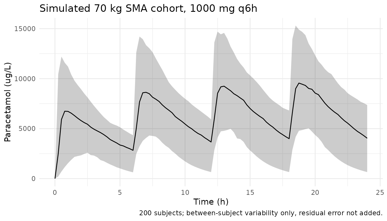
Assumptions and deviations
-
Molar amount scale (determined, not stated). Zhao
2025 does not state whether its compartments carry moles or
paracetamol-equivalent mass. The model file uses
units$dosing = "umol"/units$concentration = "umol/L", determined from the paper’s own supplementary Table S2 as shown in the “Concentration scale” section above (1-3% agreement on all three metabolite:parent AUC ratios, versus 43-111% error for a mass-equivalent reading). This matches the sibling paracetamol parent-metabolite modelvanRongen_2016_acetaminophen, which states the molar convention explicitly. Users dosing in mg must convert withdose_umol = dose_mg / 0.15116. -
Sign of two covariate exponents. The myoglobin
exponent on
CL_p/Fand the bilirubin exponent onCL_ox/Fare printed without their minus signs in the typeset Table 2 (their bootstrap CIs print in descending order, which is only possible for negative intervals). Both are encoded as negative, consistent with the “negative correlation” statements in Results section 3.3 and with the monotone half-life trends in supplementary Table S3. -
BSV is a log-scale SD, not a CV. Table 2’s “BSV
(%)” block is the log-scale standard deviation times 100, so the nlmixr2
eta variances are
(BSV / 100)^2. The determination is exact: the Discussion quotes theCL_p/FBSV as 105%, andsqrt(exp(0.862^2) - 1) = 1.050recovers that from the Table 2 value of 86.2%. - Residual error read as a standard deviation. Table 2’s “Proportional” residual block (0.28 / 0.18 / 0.22 / 0.17) is entered as proportional residual SDs, on the same standard-deviation scale as the BSV block in the same table. The supplementary paracetamol goodness-of-fit panel (observed vs individual-predicted, with the paired IWRES panel) shows relative residual scatter consistent with a ~0.28 SD rather than the ~0.53 SD that reading 0.28 as a NONMEM variance would imply.
- No baseline compartment. Pre-dose samples were below the LLOQ in most subjects and were fixed to their observed values during base-model building (Results section 3.2), so the published model carries no baseline term and neither does this implementation; all states start at zero.
- Metabolite volumes are not identifiable. They are fixed at 18% of the paracetamol volume from the literature (Methods section 2.2). The authors flag this as the probable cause of the implausibly large leftover-clearance fraction (47% in SMA, 23-27% in healthy controls, against a literature value near 4% for unchanged paracetamol; Discussion). The library model reproduces the published parameterisation without adjustment.
-
Simulated AUC compared against a cohort median.
Supplementary Tables S2 and S3 report the median AUC of 1000 simulated
subjects, while the typical-value comparison above uses zero
variability. Because
CL_p/Fcarries omega = 0.862, the median individual total clearance exceeds the typical value and the published medians therefore run a few per cent below the typical-value AUC; the 200-subject cohort check quantifies the offset. The residual disagreement is not tuned away. -
NCA half-life is not the paper’s half-life. The
half-lives tabulated in supplementary Tables S2 and S3 are
ln(2) * V / CLvalues, not terminal half-lives – the glucuronide and sulphate entries are shorter than the parent’s, which a formation-rate-limited metabolite cannot be. The comparison above therefore uses the analytic quantity; the PKNCAhalf.lifecolumn is reported separately and is not expected to match. -
Disease indicator re-expressed as
DIS_HEALTHY. The paper’s source column is the reverse-codeddiseaseindicator (1 = SMA) with the healthy controls as the reference. The model file uses the existing canonicalDIS_HEALTHY(reference category 0 = patient), shifting the structural typical tolvc = log(63.5 * 1.58)so that1 / 1.58atDIS_HEALTHY = 1restores the paper’s printed healthy-controlV_pcm/Fof 63.5 L/70 kg. This followsCleary_2023_risdiplam, which encodes the same SMA-vs-healthy contrast on the same canonical. -
MYOis a new canonical covariate column, registered ininst/references/covariate-columns.mdalongside this extraction; it joins the plasma clinical-chemistry biomarkers (ALT,AST,TBILI,ALP,LDH,CPK). -
Screened-but-unretained covariates. Sex, age, BMI,
fat-free mass, ALT, AST, ALP, LDH, creatine kinase, creatinine,
potassium and sodium are recorded in
covariatesDataExcludedbecause the paper screened them without retaining any of them; urea and glomerular filtration rate were also screened but have no unambiguous canonical column, so they are noted inpopulation$notesinstead. -
No errata identified. A search of the BJCP article
landing page, PubMed and Europe PMC for corrections to
doi:10.1002/bcp.70028returned none as of the extraction date (2026-08-17). -
No NONMEM control stream deposited. The Wiley
supplement comprises the supplementary methods (DOCX), supplementary
tables S1-S3 (DOCX) and figures S1-S9 (PDF/JPEG); no
.mod/.ctl/.lstis deposited. Every parameter value comes from Table 2 of the main publication.