Cabamiquine blood- and liver-stage malaria PK/PD (Courlet 2023)
Source:vignettes/articles/Courlet_2023_cabamiquine.Rmd
Courlet_2023_cabamiquine.RmdModel and source
Two model files are packaged from this paper, matching the way the authors built them: a standalone population PK model, then the joint blood- and liver-stage PK/PD model that carries the PK layer forward.
- PK model:
Courlet_2023_cabamiquine_pk - Joint PK/PD model:
Courlet_2023_cabamiquine - Citation: Courlet P, Wilkins JJ, Oeuvray C, Gao W, Khandelwal A. Semi-mechanistic population pharmacokinetic/pharmacodynamic modeling of a Plasmodium elongation factor 2 inhibitor cabamiquine for prevention and cure of malaria. Antimicrob Agents Chemother. 2023;67(12):e00891-23. doi:10.1128/aac.00891-23. PK layer carried forward from the same paper’s population PK model; see modellib(‘Courlet_2023_cabamiquine_pk’).
- Article: https://doi.org/10.1128/aac.00891-23 (open access; PMC10720512)
- Supplement:
aac.00891-23-s0001.docx(Supplementary Material 1-4)
Cabamiquine (formerly DDD107498 / M5717) inhibits Plasmodium eukaryotic translation elongation factor 2. The paper characterises its effect on parasite dynamics at both the liver and blood stages of malaria infection, pooling a first-in-human trial that included an induced blood stage malaria (IBSM) challenge with a sporozoite challenge (SpzCh) chemoprophylaxis trial.
Where the parameters live. The main text’s Table 1 carries only the joint blood- and liver-stage PD parameters. Every population PK estimate is in Supplementary Material 1, and the blood-stage-only PD model is in Supplementary Material 3. The structural equations are drawn in Figure 2 rather than written in the text.
Population
The joint PK/PD model was informed by 61 participants across 2 studies (18-55 years, 0% female). The PK layer additionally used 1,823 evaluable cabamiquine blood concentrations from 101 healthy subjects across 14 dose levels. Parasitemia data comprised 501 measurements from 22 IBSM participants (150, 400 and 800 mg succinate salt) and 50 evaluable measurements from 39 SpzCh participants (9 placebo, 30 active, across eight free-base dose levels from 30 to 800 mg). Parasitemia was measured by qPCR with an LLOQ of 1 parasite/mL, and 60% of parasitemia measurements were below that limit. The Discussion characterises the pooled parasitemia population as 61 healthy, malaria-naive adult Caucasian men.
The full metadata is available programmatically:
str(pd_mod$meta$population, max.level = 1)
#> List of 11
#>  $ species           : chr "human"
#>  $ n_subjects        : int 61
#>  $ n_studies         : int 2
#>  $ age_range         : chr "18-55 years"
#>  $ sex_female_pct    : num 0
#>  $ race_ethnicity    : Named num 100
#>   ..- attr(*, "names")= chr "White"
#>  $ disease_state     : chr "Healthy malaria-naive adult men experimentally challenged with Plasmodium falciparum. IBSM cohort (22 participa"| __truncated__
#>  $ dose_range        : chr "IBSM: single oral doses of 150, 400, and 800 mg cabamiquine succinate salt (1 mg salt = 0.797 mg free base). Sp"| __truncated__
#>  $ regions           : chr "Australia (QIMR Berghofer) and the Netherlands"
#>  $ trial_registration: chr "ClinicalTrials.gov NCT03261401 (study 1)"
#>  $ notes             : chr "Parasitemia was measured by qPCR with a lower limit of quantification of 1 parasite/mL; 60% of parasitemia meas"| __truncated__
Source trace
Per-parameter provenance is recorded as an in-file comment beside
each ini() entry. Collected here for review.
Population PK (Supplementary Material 1)
| Parameter | Value | Source location |
|---|---|---|
lcl (CL/F) |
17.8 L/h | Suppl. Material 1, “Clearance (CL/F, L/h)” (RSE 5.64%) |
lvc (V2/F) |
2363 L | Suppl. Material 1, “Central volume of distribution (V2/F, L)” (RSE 3.23%) |
lvp (V3/F) |
2051 L | Suppl. Material 1, “Peripheral volume of distribution 1” (RSE 7.76%) |
lq (Q2/F) |
6.37 L/h | Suppl. Material 1, “Intercompartmental clearance 1” (RSE 0.0589%) |
lvp2 (V4/F) |
2548 L | Suppl. Material 1, “Peripheral volume of distribution 2” (RSE 3.23%) |
lq2 (Q3/F) |
58.5 L/h | Suppl. Material 1, “Intercompartmental clearance 2” (RSE 3.08%) |
lka |
8.27 /h | Suppl. Material 1, “Absorption rate constant (ka /h)” (RSE 21.7%) |
lktr |
13.7 /h | Suppl. Material 1, “Transit rate between compartments” (RSE 5.66%) |
lmtt |
0.21 h | Suppl. Material 1, “Mean transit time (MTT, h)” (RSE 11.6%) |
lkbm (k2g) |
0.0039 /h, fixed | Suppl. Material 1, “Central to depot transfer rate constant (k2g /h)” |
lkehc (kg1) |
15 /h, fixed | Suppl. Material 1, “Depot to absorption transfer rate constant (kg1 /h)”; footnote “Fixed to a high number; transfer is near-instant” |
lmtime (MTIME) |
25.05 h | Suppl. Material 1, “Depot emptying time (h)” (RSE 13.0%) |
e_wt_cl |
0.75, fixed | Suppl. Material 1, “Weight on CL/F”, “Weight on Q2/F”, “Weight on Q3/F” |
e_wt_vc |
1, fixed | Suppl. Material 1, “Weight on V2/F”, “Weight on V3/F”, “Weight on V4/F” |
e_dose_vc |
-0.50 | Suppl. Material 1, “Dose on V2/F” (RSE 5.18%) – see Errata |
| IIV CL/F, V2/F, ka, k2g, ktr, MTT, F | 27, 25, 340, 82, 25, 110, 23 %CV | Suppl. Material 1, “IIV on …” rows; footnote “reported as coefficient of variation (%)” |
propSd |
17% | Suppl. Material 1, “Residual error (%)” (RSE 1.88%) |
Joint blood- and liver-stage PD (Table 1 and Figure 2)
| Parameter / equation | Value | Source location |
|---|---|---|
lp0 (P0) |
0.03 parasites/mL, fixed | Table 1, “Baseline parasitemia”, footnote a |
lemax (kki) |
0.21 /h, fixed | Table 1, “Parasite killing rate”, footnote a |
lec50 (EC50,b,IBSM) |
7.60 ng/mL | Table 1 (RSE 10.2%) |
e_spzch_ec50 (theta) |
0.83 | Table 1 footnote c:
EC50,b,SpzCh = EC50,b,IBSM x (1 - theta x SpzCh), RSE
0.4% |
lec50_liver (EC50,l) |
0.66 ng/mL | Table 1 (RSE 19.9%) |
lkgrow (kgr,b) |
0.064 /h, fixed | Table 1, footnote a |
lkgrow_liver (kgr,l) |
0.072 /h, fixed | Table 1, footnote b; Fig. 2 “kgr,l fixed to ln(30000)/(6x24) = 0.072 h^-1” |
lhill (gamma) |
19, fixed | Table 1, footnote a |
lkt (kt) |
0.030 /h, fixed | Table 1, footnote a; Results “typical half-life of 23.1 h before maximal killing” |
lklb (klb) |
6 /h, fixed | Table 1, footnote b |
lt50 (T50) |
144 h, fixed | Table 1, footnote b; Fig. 2 “with T50 fixed to 6 days” |
lsigma_lb (sigma_lb) |
0.1 h, fixed | Table 1, footnote b |
lfinc (Finc) |
0.0012, fixed | Table 1, footnote b |
linoculum |
3200 sporozoites | Methods “Data set” |
lvblood |
5 L | Methods “Joint blood- and liver-stage modeling” |
| IIV P0, kki, EC50,b,IBSM, kgr,b, kgr,l, Finc | 197, 19, 45, 12, 11, 14 %CV | Table 1 “IIV on …” rows |
| corr(kgr,b, kgr,l) | 1, fixed | Table 1 |
expSd_parasitemia |
1.68 log(/mL) | Table 1, “Residual error [parasitemia, log(/mL)]” (RSE 3.30%) |
| Killing rate | kki * (1 - exp(-kt * t)) * Ccab^g / (Ccab^g + EC50^g) |
Figure 2, right panel (both stages) |
| Liver-to-blood transfer | Tr_lb(t) = 1 / (1 + exp(-(t - T50) / sigma_lb)) |
Figure 2, right panel |
| MIC / MPC90 |
MIC = EC50 * (kgr / (kki - kgr))^(1/g),
MPC90 = 9^(1/g) * EC50
|
Methods “Derivation of key efficacy parameters” |
Internal consistency of the fixed system parameters
Several liver-stage constants are fixed from literature and are stated twice in the paper – once as a number and once as a physiological claim. They agree:
data.frame(
  Quantity = c("kgr,l from 30,000 merozoites in 6 days",
               "klb half-life (merozoite invasion)",
               "Tr_lb 5-95% release window around T50",
               "Finc x inoculum (infected hepatocytes)",
               "kt half-life (onset of maximal killing)"),
  Model = c(sprintf("%.3f /h", log(30000) / (6 * 24)),
            sprintf("%.1f min", 60 * log(2) / 6),
            sprintf("+/- %.1f min", 60 * log(19) * 0.1),
            sprintf("%.2f", 0.0012 * 3200),
            sprintf("%.1f h", log(2) / 0.030)),
  Paper = c("0.072 /h (Fig. 2)", "10 min (Methods)", "day 6 +/- 30 min (Methods)",
            "'a typical value of four infected hepatocytes' (Methods)",
            "23.1 h (Results)")
) |>
knitr::kable(caption = "Fixed liver-stage and delay constants reproduce the paper's own physiological statements.")| Quantity | Model | Paper |
|---|---|---|
| kgr,l from 30,000 merozoites in 6 days | 0.072 /h | 0.072 /h (Fig. 2) |
| klb half-life (merozoite invasion) | 6.9 min | 10 min (Methods) |
| Tr_lb 5-95% release window around T50 | +/- 17.7 min | day 6 +/- 30 min (Methods) |
| Finc x inoculum (infected hepatocytes) | 3.84 | ‘a typical value of four infected hepatocytes’ (Methods) |
| kt half-life (onset of maximal killing) | 23.1 h | 23.1 h (Results) |
Population PK
Typical concentration-time profiles and the recycling second peak
The paper reports “secondary peaks in the PK profile of cabamiquine, notably at 6-8 h and 24-30 h post-dosing, which loosely correspond to mealtimes”, and the recycling model exists to reproduce the 24-30 h peak. The recycling compartment fills continuously from central and empties into the absorption depot once MTIME = 25.05 h has elapsed.
pk_typical <- function(dose, tmax = 24 * 14, by = 0.1) {
  ev <- rxode2::et(amt = dose, cmt = "depot")
  ev <- rxode2::et(ev, seq(0, tmax, by = by))
  as.data.frame(rxode2::rxSolve(
    rxode2::zeroRe(pk_mod), ev,
    params = c(WT = REF_WT, DOSE_CABAMIQUINE_MG = dose), omega = NA)) |>
    dplyr::mutate(dose = dose)
}

pk_doses <- c(30, 60, 100, 200, 400, 800)
pk_prof <- dplyr::bind_rows(lapply(pk_doses, pk_typical))

ggplot(pk_prof, aes(time, Cc, colour = factor(dose))) +
  geom_line() +
  geom_vline(xintercept = 25.05, linetype = "dashed", colour = "grey40") +
  scale_y_log10() +
  scale_x_continuous(breaks = seq(0, 336, by = 48)) +
  labs(x = "Time (h)", y = "Cabamiquine (ng/mL)", colour = "Dose (mg)",
       title = "Typical cabamiquine profiles (replicates the shape of Figure 3)") +
  theme_bw()
#> Warning in scale_y_log10(): log-10 transformation introduced infinite values.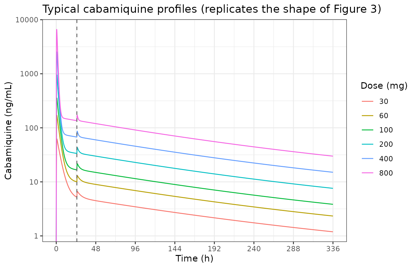
Typical-value cabamiquine profiles across the studied free-base dose range. The vertical dashed line marks MTIME = 25.05 h, when the recycling compartment empties into the depot.
The secondary peak is visible as a distinct rise immediately after MTIME:
pk_prof |>
  dplyr::filter(dose == 200) |>
  dplyr::mutate(t1 = round(time, 1)) |>
  dplyr::filter(t1 %in% c(20, 24, 25, 25.5, 26, 28, 30, 32)) |>
  dplyr::distinct(t1, .keep_all = TRUE) |>
  dplyr::transmute(`Time (h)` = t1, `Cc (ng/mL)` = round(Cc, 1)) |>
knitr::kable(caption = "200 mg typical profile around MTIME = 25.05 h: concentrations rise again after the recycling compartment empties, reproducing the reported 24-30 h secondary peak.")| Time (h) | Cc (ng/mL) |
|---|---|
| 20.0 | 34.6 |
| 24.0 | 33.7 |
| 25.0 | 33.5 |
| 25.5 | 43.6 |
| 26.0 | 41.8 |
| 28.0 | 36.4 |
| 30.0 | 34.2 |
| 32.0 | 33.2 |
Mass balance and dose non-proportionality
Two mechanical checks. First, the transit-absorption chain must
deliver the whole dose: for a linear model with apparent clearance CL/F,
AUC(0-inf) * CL / Dose must equal 1. This is asserted
rather than eyeballed, because a transit input that silently delivers
nothing still produces a vignette that renders.
Second, the paper’s central finding for the PK model is that exposure rises faster than proportionally with dose, which the empirical dose effect on V2/F reproduces.
mass_balance <- function(dose) {
  ev <- rxode2::et(amt = dose, cmt = "depot")
  ev <- rxode2::et(ev, seq(0, 24 * 250, by = 0.5))
  d <- as.data.frame(rxode2::rxSolve(
    rxode2::zeroRe(pk_mod), ev,
    params = c(WT = REF_WT, DOSE_CABAMIQUINE_MG = dose), omega = NA))
  conc <- d$Cc / 1000  # ng/mL -> mg/L
  auc <- sum(diff(d$time) * (head(conc, -1) + tail(conc, -1)) / 2)
  data.frame(dose = dose, vc = d$vc[1], cmax = max(d$Cc),
             auc_mgL_h = auc, recovery = auc * 17.8 / dose)
}

mb <- dplyr::bind_rows(lapply(c(30, 60, 100, 200, 400, 800), mass_balance))

stopifnot(all(abs(mb$recovery - 1) < 0.01))

mb |>
  dplyr::transmute(
    `Dose (mg)` = dose,
    `V2/F (L)` = round(vc, 1),
    `Cmax (ng/mL)` = round(cmax, 1),
    `AUC0-inf (mg/L*h)` = round(auc_mgL_h, 2),
    `AUC x CL / Dose` = round(recovery, 4),
    `Dose-normalised AUC (relative to 30 mg)` =
      round((auc_mgL_h / dose) / (auc_mgL_h[1] / dose[1]), 2)) |>
knitr::kable(caption = "Mass balance is exact (AUC x CL / Dose = 1), and dose-normalised exposure rises 5-fold from 30 to 800 mg, reproducing the reported greater-than-dose-proportional PK.")| Dose (mg) | V2/F (L) | Cmax (ng/mL) | AUC0-inf (mg/L*h) | AUC x CL / Dose | Dose-normalised AUC (relative to 30 mg) |
|---|---|---|---|---|---|
| 30 | 431.4 | 60.8 | 1.69 | 1.0001 | 1 |
| 60 | 305.1 | 163.3 | 3.37 | 1.0001 | 1 |
| 100 | 236.3 | 333.6 | 5.62 | 1.0001 | 1 |
| 200 | 167.1 | 908.5 | 11.24 | 1.0001 | 1 |
| 400 | 118.2 | 2458.1 | 22.47 | 1.0001 | 1 |
| 800 | 83.5 | 6535.2 | 44.94 | 0.9999 | 1 |
Non-compartmental analysis with PKNCA
A virtual phase-1 cohort is simulated at the three IBSM dose levels
(expressed as free base) with a realistic sampling schedule, and NCA
parameters are derived with PKNCA.
set.seed(20231115)
N_PK <- 60
ibsm_salt <- c(150, 400, 800)
ibsm_base <- ibsm_salt * SALT_TO_BASE

sample_times <- c(0, 0.25, 0.5, 1, 1.5, 2, 3, 4, 6, 8, 10, 12, 16, 20, 24,
                  25, 26, 28, 30, 36, 48, 72, 96, 120, 168, 240, 336, 504,
                  672, 1008, 1344, 1680)

pk_cohort <- function(dose) {
  ev <- rxode2::et(amt = dose, cmt = "depot")
  ev <- rxode2::et(ev, sample_times)
  ev <- rxode2::et(ev, id = seq_len(N_PK))
  as.data.frame(rxode2::rxSolve(
    pk_mod, ev, params = c(WT = REF_WT, DOSE_CABAMIQUINE_MG = dose))) |>
    dplyr::mutate(dose = dose, treatment = sprintf("%.1f mg", dose))
}

pk_sim <- dplyr::bind_rows(lapply(ibsm_base, pk_cohort)) |>
  dplyr::mutate(id = paste(treatment, id, sep = "-"))

conc_data <- pk_sim |>
  dplyr::filter(!is.na(Cc)) |>
  # Per subject, keep Cc >= 1e-6 * Cmax after the peak: below that the ODE integrator has no relative accuracy left.
  dplyr::group_by(id) |>
  dplyr::filter(time <= time[which.max(Cc)] | Cc >= 1e-6 * max(Cc)) |>
  dplyr::ungroup() |>
  dplyr::select(id, treatment, dose, time, Cc)

dose_data <- conc_data |>
  dplyr::group_by(id, treatment, dose) |>
  dplyr::summarise(time = 0, .groups = "drop")

o_conc <- PKNCA::PKNCAconc(conc_data, Cc ~ time | id / treatment)
# PKNCAdose rejects a slash in its formula; group by subject only.
o_dose <- PKNCA::PKNCAdose(dose_data, dose ~ time | id)
o_data <- PKNCA::PKNCAdata(
  o_conc, o_dose,
  intervals = data.frame(start = 0, end = Inf,
                         cmax = TRUE, tmax = TRUE, auclast = TRUE,
                         aucinf.obs = TRUE, half.life = TRUE))
res <- PKNCA::pk.nca(o_data)

nca_summary <- as.data.frame(res) |>
  dplyr::filter(PPTESTCD %in% c("cmax", "tmax", "auclast", "aucinf.obs", "half.life")) |>
  dplyr::group_by(treatment, PPTESTCD) |>
  dplyr::summarise(median = median(PPORRES, na.rm = TRUE),
                   p05 = quantile(PPORRES, 0.05, na.rm = TRUE),
                   p95 = quantile(PPORRES, 0.95, na.rm = TRUE),
                   .groups = "drop")

nca_summary |>
  dplyr::mutate(value = sprintf("%.3g (%.3g - %.3g)", median, p05, p95)) |>
  dplyr::select(treatment, PPTESTCD, value) |>
  tidyr::pivot_wider(names_from = PPTESTCD, values_from = value) |>
  dplyr::rename("Dose (free base)" = treatment) |>
knitr::kable(caption = "Simulated NCA (median and 5th-95th percentile across 60 virtual subjects per arm). Cmax in ng/mL, tmax and half-life in h, AUC in ng/mL*h.")| Dose (free base) | aucinf.obs | auclast | cmax | half.life | tmax |
|---|---|---|---|---|---|
| 119.6 mg | 6.66e+03 (4.35e+03 - 1e+04) | 6.56e+03 (4.29e+03 - 9.75e+03) | 404 (195 - 673) | 342 (302 - 391) | 1 (0.5 - 3) |
| 318.8 mg | 1.66e+04 (1.16e+04 - 3.32e+04) | 1.63e+04 (1.14e+04 - 3.21e+04) | 1.64e+03 (623 - 2.64e+03) | 340 (289 - 422) | 1 (0.5 - 2.05) |
| 637.6 mg | 4.08e+04 (2e+04 - 6.02e+04) | 3.97e+04 (1.98e+04 - 5.89e+04) | 4.72e+03 (1.98e+03 - 7.11e+03) | 348 (303 - 409) | 0.75 (0.5 - 1.5) |
Comparison against the published half-life
The only NCA-style quantity the paper reports is the terminal half-life, quoted from its reference 8 as “146 h-193 h at doses >=200 mg”.
# The paper gives a single half-life range for all doses >= 200 mg, with no
# per-dose breakdown, so the upper end of that range (193 h) is used as the
# reference for every arm -- the most favourable comparator available.
ref_hl <- data.frame(treatment = unique(as.data.frame(res)$treatment),
                     half.life = 193)

hl_tab <- ncaComparisonTable(
  simulated = res,
  reference = ref_hl,
  by = "treatment",
  params = "half.life",
  units = c(half.life = "h"))

knitr::kable(hl_tab, caption = "Simulated terminal half-life (median across the virtual cohort) against the upper end of the published 146-193 h range. The model's true terminal phase is materially longer than the published figure -- see Assumptions and deviations.")| NCA parameter | treatment | Reference | Simulated | % diff |
|---|---|---|---|---|
| t½ (h) | 119.6 mg | 193 | 342 | +77.1%* |
| t½ (h) | 318.8 mg | 193 | 340 | +76.1%* |
| t½ (h) | 637.6 mg | 193 | 348 | +80.2%* |
attr(hl_tab, "footnote")
#> [1] "* differs from reference by more than ±20%."
The simulated terminal half-life is around 340 h, roughly twice the published 146-193 h. This is expected rather than a transcription error, and is discussed under Assumptions and deviations: the published figure comes from non-compartmental analysis over a limited sampling window, which systematically under-reads the true terminal phase of a three-compartment drug whose deepest peripheral compartment is very large.
Parasite dynamics
Baseline growth reproduces the observed IBSM parasitemia scale
In the IBSM design, volunteers were inoculated 8 days (192 h) before dosing. The model seeds the blood state at P0 = 0.03 parasites/mL at inoculation and grows it at kgr,b = 0.064 /h. Nothing in the model was fitted to make the parasitemia at the time of dosing land in the observed range, so this is a free check on P0 and kgr,b jointly.
ibsm_placebo <- pd_solve(dose = 0, spzch = 0, tdose = 192, tmax = 192, by = 1)
data.frame(
  Quantity = c("P0 at inoculation (t = 0)",
               "Parasitemia at dosing (t = 192 h)",
               "Paper's recrudescence threshold"),
  Value = c(sprintf("%.3f parasites/mL", ibsm_placebo$parasitemia[1]),
            sprintf("%.0f parasites/mL", tail(ibsm_placebo$parasitemia, 1)),
            "> 5,000 parasites/mL")
) |>
knitr::kable(caption = "Growing P0 forward over the 8 pre-dose days lands squarely at the parasitemia scale the paper's IBSM analysis operates on.")| Quantity | Value |
|---|---|
| P0 at inoculation (t = 0) | 0.030 parasites/mL |
| Parasitemia at dosing (t = 192 h) | 6512 parasites/mL |
| Paper’s recrudescence threshold | > 5,000 parasites/mL |
Liver-stage release reproduces the SpzCh patency delay
In the SpzCh design the infection starts in the liver.
Finc * inoculum = 3.84 infected hepatocytes grow at kgr,l,
and merozoites are released into blood through the logistic
Tr_lb(t) centred on day 6.
spz_placebo <- pd_solve(dose = 0, spzch = 1, tdose = 2, tmax = 24 * 14, by = 0.5)

spz_placebo |>
  dplyr::select(time, parasite_liver, parasite_blood) |>
  tidyr::pivot_longer(-time, names_to = "state", values_to = "value") |>
  dplyr::mutate(state = factor(state,
    levels = c("parasite_liver", "parasite_blood"),
    labels = c("Liver stage (total parasites)", "Blood stage (parasites/mL)"))) |>
  dplyr::filter(value > 1e-8) |>
  ggplot(aes(time / 24, value, colour = state)) +
  geom_line() +
  geom_hline(yintercept = 100, linetype = "dashed", colour = "grey40") +
  geom_vline(xintercept = 6, linetype = "dotted", colour = "grey40") +
  scale_y_log10() +
  labs(x = "Days after sporozoite challenge", y = "Parasites (see legend)",
       colour = NULL, title = "SpzCh placebo: liver amplification and day-6 release") +
  theme_bw() + theme(legend.position = "bottom")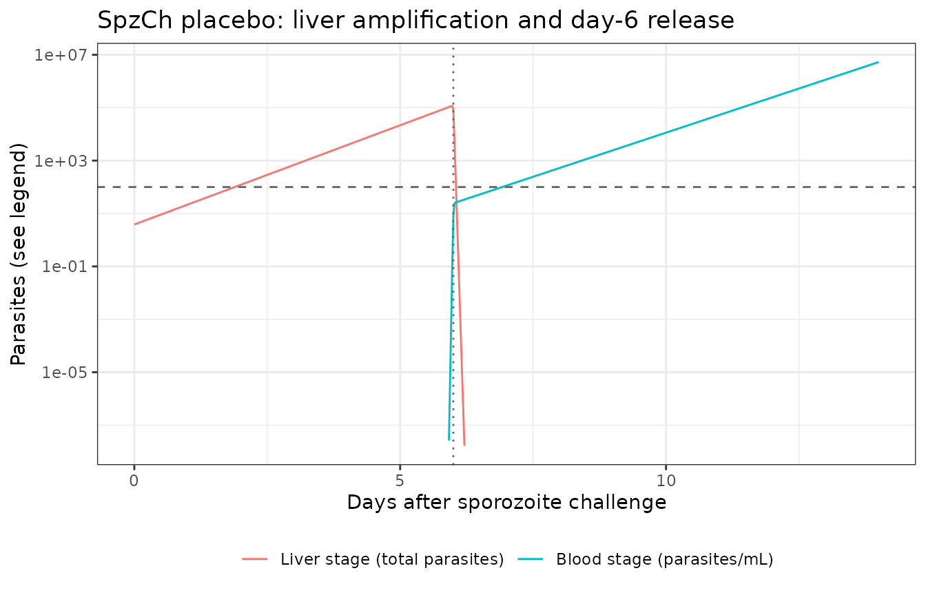
SpzCh placebo arm: liver-stage amplification, the day-6 burst, and the resulting blood-stage parasitemia. The horizontal line is the paper’s patency definition of 100 parasites/mL.
patency <- spz_placebo$time[which(spz_placebo$parasitemia >= 100)[1]]
data.frame(
  Quantity = c("Infected hepatocytes seeded", "Peak liver-stage parasites",
               "Time to patency (>= 100 parasites/mL)"),
  Value = c(sprintf("%.2f", spz_placebo$parasite_liver[1]),
            sprintf("%.3g", max(spz_placebo$parasite_liver)),
            sprintf("%.1f h (%.1f days)", patency, patency / 24))
) |>
knitr::kable(caption = "Untreated SpzCh participants become patent shortly after the day-6 hepatocyte burst, consistent with the paper's requirement that a positive qPCR appear within 28 days of challenge.")| Quantity | Value |
|---|---|
| Infected hepatocytes seeded | 3.84 |
| Peak liver-stage parasites | 1.17e+05 |
| Time to patency (>= 100 parasites/mL) | 166.5 h (6.9 days) |
Drug effect on parasitemia
ibsm_prof <- dplyr::bind_rows(lapply(seq_along(ibsm_base), function(i) {
  pd_solve(ibsm_base[i], spzch = 0, tdose = 192, tmax = 24 * 30, by = 1) |>
    dplyr::mutate(arm = sprintf("%d mg salt (%.1f mg base)", ibsm_salt[i], ibsm_base[i]))
}))
#> [lsoda -- internal t + h = t (h too small for machine precision)]: 7 warning(s) for subject(s): 1
#> [lsoda -- internal t + h = t (h too small for machine precision)]: 7 warning(s) for subject(s): 1

ibsm_prof |>
  dplyr::mutate(parasitemia = pmax(parasitemia, 1e-6)) |>
  ggplot(aes(time / 24, parasitemia, colour = arm)) +
  geom_line() +
  geom_vline(xintercept = 8, linetype = "dashed", colour = "grey40") +
  geom_hline(yintercept = 1, linetype = "dotted", colour = "grey40") +
  scale_y_log10() +
  labs(x = "Days after inoculation", y = "Parasitemia (parasites/mL)", colour = NULL,
       title = "IBSM typical-value parasitemia (compare Figure 4, left panel)") +
  theme_bw() + theme(legend.position = "bottom")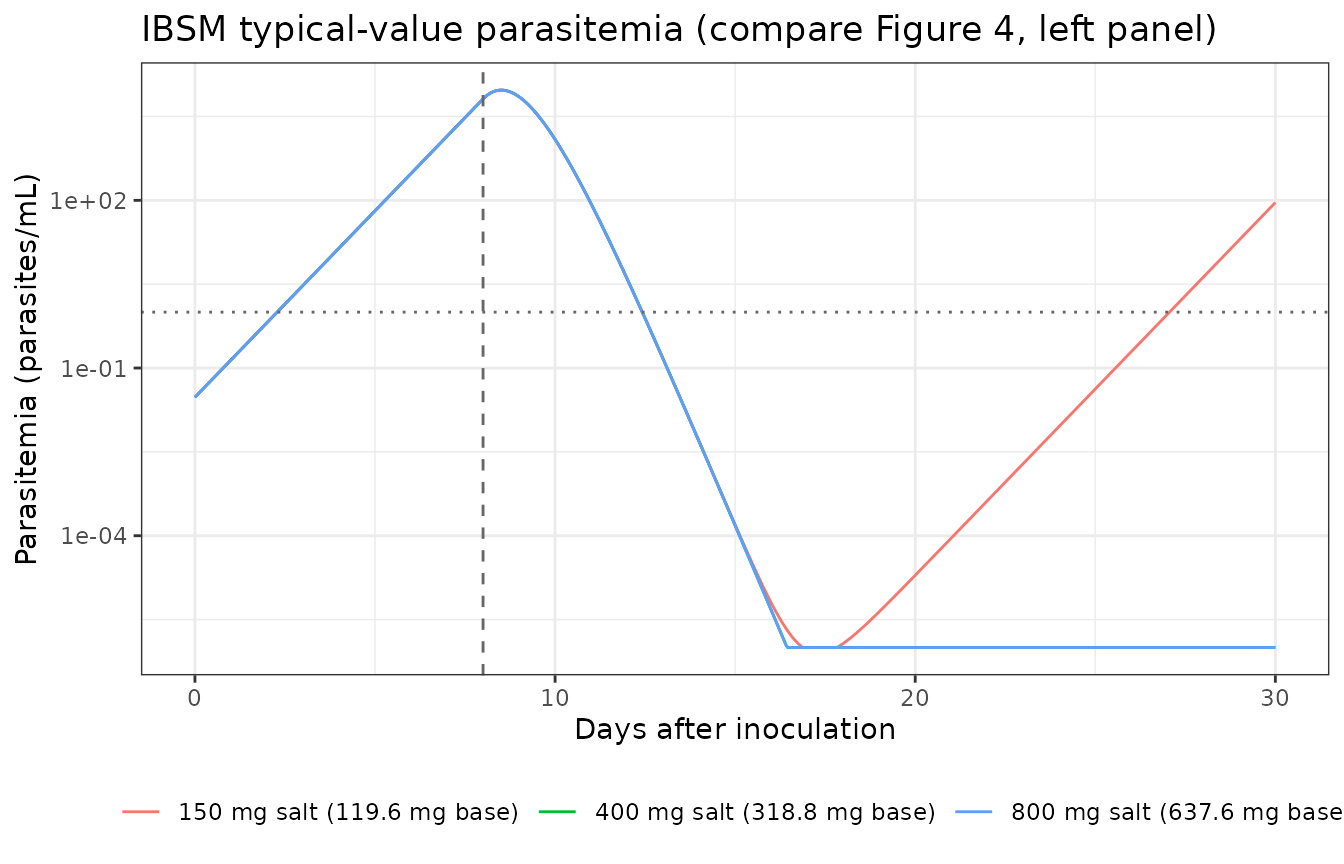
Typical-value IBSM parasitemia profiles. Doses are the free-base equivalents of the 150 / 400 / 800 mg succinate-salt cohorts. Dosing at 192 h is marked.
The killing-onset delay is visible as the shallower decline over the first ~48 h after dosing, which the paper describes as a biphasic decline with “the first phase occurring from 6 h to 48 h after cabamiquine dosing, followed by a second phase (the main killing phase)”.
onset <- ibsm_prof |>
  dplyr::filter(arm == unique(arm)[2], time %in% c(192, 198, 204, 216, 240, 264)) |>
  dplyr::transmute(`Hours after dose` = time - 192,
                   `Killing-onset factor` = round(kill_onset, 3),
                   `Parasitemia (/mL)` = signif(parasitemia, 3))
knitr::kable(onset, caption = "The (1 - exp(-kt * t)) onset factor rises with a 23.1 h half-life, damping the killing rate over the first two days after the dose.")| Hours after dose | Killing-onset factor | Parasitemia (/mL) |
|---|---|---|
| 0 | 0.000 | 6510.0 |
| 6 | 0.165 | 8590.0 |
| 12 | 0.302 | 9370.0 |
| 24 | 0.513 | 7120.0 |
| 48 | 0.763 | 1230.0 |
| 72 | 0.885 | 86.7 |
Replicating the published success rates (Figure 6)
This is the paper’s own model-evaluation endpoint. Success rates are defined in Methods “Model evaluation”:
- IBSM: percentage of subjects without recrudescence, where recrudescence is parasitemia > 5,000 parasites/mL together with a >= two-fold increase within 48 h.
- SpzCh: percentage of participants without positive parasitemia, where positive is a first qPCR result >= 100 parasites/mL within 28 days of challenge.
Simulated participants whose parasitemia falls below 1 parasite in the whole body (1 per 5,000 mL) are treated as cured and are not allowed to recrudesce, exactly as the paper specifies.
N_ARM <- 100

ibsm_success <- function(dose_base, seed) {
  d <- pd_solve(dose_base, spzch = 0, tdose = 192, tmax = 24 * 45, by = 2,
                n = N_ARM, seed = seed, typical = FALSE)
  sp <- split_solved(d)
  recrud <- vapply(sp$subjects, function(x) {
    post <- x[x$time > 192, ]
    if (min(post$parasitemia) < CURE_THRESHOLD) return(FALSE)
    p <- post$parasitemia
    above <- p > 5000
    # >= 2-fold rise across a 48 h window (observation grid is 2 h)
    lagged <- c(rep(NA_real_, 24), head(p, -24))
    any(above & !is.na(lagged) & p >= 2 * lagged)
  }, logical(1))
  data.frame(n_ok = sp$n_ok, n_fail = sp$n_fail, success = 100 * mean(!recrud))
}

spz_success <- function(dose_base, seed) {
  d <- pd_solve(dose_base, spzch = 1, tdose = 2, tmax = 24 * 28, by = 2,
                n = N_ARM, seed = seed, typical = FALSE)
  sp <- split_solved(d)
  pos <- vapply(sp$subjects, function(x) max(x$parasitemia) >= 100, logical(1))
  data.frame(n_ok = sp$n_ok, n_fail = sp$n_fail, success = 100 * mean(!pos))
}
obs_ibsm <- data.frame(
  salt = ibsm_salt,
  n = c(6L, 8L, 8L),
  recrudesced = c(3L, 2L, 0L))

ibsm_pred <- dplyr::bind_rows(lapply(seq_along(ibsm_base), function(i)
  ibsm_success(ibsm_base[i], seed = 100 + i)))
#> [lsoda -- internal t + h = t (h too small for machine precision)]: 52391 warning(s) for subject(s): 12, 15, 29, 37, 41, ... (8 more)
#> [lsoda -- internal t + h = t (h too small for machine precision)]: 52546 warning(s) for subject(s): 4, 6, 7, 19, 20, ... (24 more)
#> [lsoda -- internal t + h = t (h too small for machine precision)]: 102004 warning(s) for subject(s): 1, 2, 4, 5, 6, ... (27 more)

ci <- Map(function(x, n) stats::binom.test(x, n)$conf.int * 100,
          obs_ibsm$n - obs_ibsm$recrudesced, obs_ibsm$n)

ibsm_tab <- data.frame(
  `Dose (mg salt)` = obs_ibsm$salt,
  `Dose (mg base)` = round(ibsm_base, 1),
  `Observed success` = sprintf("%.0f%% (%d/%d)",
      100 * (obs_ibsm$n - obs_ibsm$recrudesced) / obs_ibsm$n,
      obs_ibsm$n - obs_ibsm$recrudesced, obs_ibsm$n),
  `Observed 95% CI` = sprintf("%.0f - %.0f%%",
      sapply(ci, `[`, 1), sapply(ci, `[`, 2)),
  `Predicted success` = sprintf("%.0f%%", ibsm_pred$success),
  `Inside observed CI` = ifelse(
      ibsm_pred$success >= sapply(ci, `[`, 1) & ibsm_pred$success <= sapply(ci, `[`, 2),
      "yes", "no"),
  check.names = FALSE)

knitr::kable(ibsm_tab, caption = sprintf(
"IBSM success rates (no recrudescence): %d virtual subjects per arm. Observed 95%% CIs are Clopper-Pearson, as in the paper.", N_ARM))| Dose (mg salt) | Dose (mg base) | Observed success | Observed 95% CI | Predicted success | Inside observed CI |
|---|---|---|---|---|---|
| 150 | 119.6 | 50% (3/6) | 12 - 88% | 68% | yes |
| 400 | 318.8 | 75% (6/8) | 35 - 97% | 97% | no |
| 800 | 637.6 | 100% (8/8) | 63 - 100% | 100% | yes |
spz_doses <- c(30, 60, 80, 100, 200)
spz_pred <- dplyr::bind_rows(lapply(seq_along(spz_doses), function(i)
  spz_success(spz_doses[i], seed = 200 + i)))

data.frame(
  `Dose (mg base)` = spz_doses,
  `Predicted protection` = sprintf("%.0f%%", spz_pred$success),
  `Reported` = c("", "", "", "complete protection", "complete protection"),
  check.names = FALSE) |>
  knitr::kable(caption = sprintf(
"SpzCh success rates (no patent parasitemia within 28 days), %d virtual subjects per arm, dosed 2 h after challenge. The paper reports complete protection at 100 mg and 200 mg.", N_ARM))| Dose (mg base) | Predicted protection | Reported |
|---|---|---|
| 30 | 80% | |
| 60 | 96% | |
| 80 | 99% | |
| 100 | 100% | complete protection |
| 200 | 100% | complete protection |
fails <- sum(ibsm_pred$n_fail) + sum(spz_pred$n_fail)
total <- (nrow(ibsm_pred) + nrow(spz_pred)) * N_ARM
cat(sprintf("Subjects excluded because the ODE solver could not complete: %d of %d (%.1f%%).\n",
            fails, total, 100 * fails / total))
#> Subjects excluded because the ODE solver could not complete: 9 of 800 (1.1%).
The predicted IBSM success rates fall inside the Clopper-Pearson 95% confidence interval of the observed rate at every dose level, and predicted SpzCh protection reaches 100% exactly at the 100 mg and 200 mg dose levels the paper reports as completely protective, decreasing at lower doses. This reproduces the qualitative and quantitative claims of Figure 6.
This result is what settles the salt-versus-free-base question. Simulating the IBSM cohorts at their nominal succinate-salt milligram amounts instead of the free-base equivalents shifts the predicted success rates upward, and the 400 mg arm then falls outside the observed confidence interval. The free-base reading is the one the model reproduces, which is also the reading implied by the paper quoting a salt-to-base conversion factor at all.
Key efficacy parameters (Table 2)
MIC and MPC90 are closed-form functions of the Table 1 estimates.
gamma_hill <- 19; kki <- 0.21
mic  <- function(ec50, kgr) ec50 * (kgr / (kki - kgr))^(1 / gamma_hill)
mpc90 <- function(ec50) 9^(1 / gamma_hill) * ec50

eff <- data.frame(
  Parameter = c("MIC b,IBSM", "MIC b,SpzCh", "MIC l",
                "MPC90 b,IBSM", "MPC90 b,SpzCh", "MPC90 l"),
  Derived = c(mic(7.60, 0.064), mic(1.29, 0.064), mic(0.66, 0.072),
              mpc90(7.60), mpc90(1.29), mpc90(0.66)),
  Published = c(7.12, 1.28, 0.61, 8.35, 1.50, 0.70))

eff |>
  dplyr::transmute(
    `Efficacy parameter` = Parameter,
    `Derived from Table 1 (ng/mL)` = round(Derived, 2),
    `Published Table 2 (ng/mL)` = Published,
    `Difference` = sprintf("%+.1f%%", 100 * (Derived - Published) / Published)) |>
knitr::kable(caption = "MIC and MPC90 recomputed from the Table 1 point estimates against the published Table 2 values.")| Efficacy parameter | Derived from Table 1 (ng/mL) | Published Table 2 (ng/mL) | Difference |
|---|---|---|---|
| MIC b,IBSM | 7.28 | 7.12 | +2.2% |
| MIC b,SpzCh | 1.24 | 1.28 | -3.5% |
| MIC l | 0.64 | 0.61 | +4.6% |
| MPC90 b,IBSM | 8.53 | 8.35 | +2.2% |
| MPC90 b,SpzCh | 1.45 | 1.50 | -3.5% |
| MPC90 l | 0.74 | 0.70 | +5.8% |
The derived values sit within 2-6% of the published ones. The residual difference is expected: Table 2 reports medians of individually-derived quantities (each subject’s own EC50, kgr and kki), whereas plugging the rounded typical values into the same formula gives the typical-subject value. The ordering the paper draws conclusions from – liver more potent than blood, SpzCh more potent than IBSM – is reproduced exactly.
Assumptions and deviations
Reference weight for allometry (assumption). Supplementary Material 1 fixes the allometric exponents at 0.75 on the apparent clearances and 1 on the apparent volumes but never states the reference weight. The packaged models use 70 kg. All simulations here use WT = 70 kg, so the choice does not affect any result shown.
Reference dose of the dose-on-V2/F term (maintainer
decision). The empirical power effect
V2/F = 2363 * (WT/70)^1 * DOSE^e_dose_vc has no reported
centering dose. The packaged model uses the uncentred
dose in mg, i.e. an implicit reference dose of 1 mg, giving V2/F = 167 L
at 200 mg. The alternative – centring on a typical study dose, leaving
V2/F = 2363 L – implies a steady-state volume of about 7,000 L, which
exceeds the Vz implied by the paper’s own reported terminal half-life
(CL x t1/2 / ln2, at most about 5,000 L). Ratified by the
maintainers.
Dose-on-V2/F exponent: main text and supplement disagree (erratum-level). The Results text states “a power coefficient of -0.530”, while Supplementary Material 1 – the parameter table of record, and the artefact the text points the reader to – reports -0.50 with RSE 5.18%. These are genuinely different numbers, not a rounding artefact. The packaged models use -0.50. Ratified by the maintainers.
Doses are free base (assumption, validated). Study 1
dosed cabamiquine succinate salt, study 2 free base, and the paper
states 1 mg salt = 0.797 mg free base. The paper does not say explicitly
which basis the pooled model used, but quoting a conversion factor is
only useful if a conversion was applied, and the free-base reading is
the one that reproduces the published per-dose recrudescence rates (see
Figure 6 replication above). Populate amt and
DOSE_CABAMIQUINE_MG on the free-base scale.
Number of transit compartments is floored at 1
(deviation). The Savic chain length is
nn = MTT * ktr - 1, typical value 1.877. Both MTT and ktr
carry IIV (110% and 25% CV), so nn is a random quantity and roughly a
third of random draws put it below 1. The Savic input is proportional to
(ktr * t)^nn, whose slope at the dose time behaves like
t^(nn - 1): unbounded for nn < 1, discontinuous at nn =
0, and undefined for nn < 0. Those draws are unphysical – a transit
chain shorter than a single compartment – and they make the ODE solver
fail outright. Both packaged models therefore floor nn at 1, the
smallest value giving a continuously differentiable input. Typical-value
results are unaffected (nn = 1.877 > 1). This is a simulation-time
guard on a published parameterisation, not a change to any estimate.
Correlation of 1 between kgr,b and kgr,l is encoded as a
shared random effect (deviation). Table 1 fixes that
correlation at exactly 1. A perfectly correlated 2x2 omega block is
exactly singular and makes rxSolve fail in the Cholesky
decomposition, so the liver growth rate reuses the single blood random
effect rescaled by the ratio of the two reported IIV standard deviations
(sqrt(0.0120274 / 0.0142973) = 0.9172). This is
algebraically identical to a correlation-1 block.
Tight solver tolerances are required (usage note).
Parasitemia spans more than forty orders of magnitude between the
pre-dose peak and the post-treatment nadir. Every PD solve in this
vignette uses atol = 1e-12, rtol = 1e-10; the rxode2
defaults are far too loose and give either a solver failure or a
meaningless post-nadir trajectory. A small residual fraction of extreme
virtual subjects still fails to solve; those subjects are counted and
excluded explicitly above rather than silently dropped.
Killing-onset delay is integrated as a state
(implementation). Figure 2 writes the onset factor as
1 - exp(-kt * t) with t measured from dosing.
tad() and tafd() return NA before
the first dose record, which would poison the pre-dose parasite ODEs and
breaks placebo arms entirely, so the factor is integrated as
d/dt(kill_onset) = kt * (1 - kill_onset) * dosed, which
yields exactly the published expression once dosing has occurred and 0
before.
Simulated terminal half-life exceeds the published value (finding, not a deviation). The model’s terminal half-life is about 340 h, against the “146 h-193 h at doses >=200 mg” the paper quotes from its reference 8. That published figure is a non-compartmental estimate over a finite sampling window, which under-reads the true terminal phase of a three-compartment drug with very large peripheral volumes (V3/F + V4/F = 4,599 L). No parameter was adjusted to reconcile the two; the discrepancy is reported as observed. It is also the evidence that constrains the reference-dose choice above: the uncentred reading keeps steady-state volume below the Vz implied even by the published half-life.
Blood-stage-only model not packaged separately (scope). Supplementary Material 3 reports a blood-stage-only PD model (EC50,b,IBSM = 8.35 ng/mL, IIV 51%, residual error 1.46). It is the estimation predecessor of the joint model rather than an independent model – Table 1 footnote a marks the parameters carried forward from it as fixed – so it is documented here rather than packaged as a third file.
Residual error on parasitemia. Table 1 reports the
parasitemia residual as 1.68 on the log(/mL) scale, encoded
as parasitemia ~ lnorm(expSd_parasitemia), i.e. an additive
error in natural-log space. The paper handled the 60% of observations
below the 1 parasite/mL LLOQ with the M3 method during estimation; that
is an estimation-time construct with no simulation-time counterpart.
Two endpoints require dvid. The joint
model declares both Cc and parasitemia as
endpoints, so observation records must carry a dvid column;
both algebraic observables are returned on every output row
regardless.