Translational TfR-mediated brain delivery of antibodies (Muliaditan 2025)
Source:vignettes/articles/Muliaditan_2025_mab_mpbpk.Rmd
Muliaditan_2025_mab_mpbpk.RmdModel and source
- Citation: Muliaditan M, van Steeg TJ, Avery LB, Sun W, Hammond TR, Hijdra D, Choi SL, Pillai N, Leksa NC, Mavroudis PD. Translational minimal physiologically based pharmacokinetic model for transferrin receptor-mediated brain delivery of antibodies. mAbs. 2025;17(1):2515414.
- DOI: https://doi.org/10.1080/19420862.2025.2515414
- PMID: 40568753
The paper develops a minimal physiologically based
pharmacokinetic (mPBPK) model for monoclonal antibody (mAb)
delivery to the brain via transferrin-receptor (TfR) mediated
transcytosis. The mPBPK framework combines (a) the Bloomingdale 2017 mAb
mPBPK structure (plasma, lumped tissue vascular / endosomal /
interstitial spaces, brain vascular, blood-brain barrier (BBB) endosome,
brain ISF, blood-CSF barrier (BCSFB) endosome, CSF, lymph, with
FcRn-mediated recycling of intact antibody from each endosomal
compartment) and (b) Chang 2022’s TfR binding sites at the plasma,
luminal BBB, luminal BCSFB, abluminal BBB (brain ISF), abluminal BCSFB
(CSF), and neuronal compartments. The bsAb-TfR complex is transcytosed
across the brain barriers at a fixed rate ktrans = 6 h^-1
and is empirically degraded at rate kint (modelled as a
binary fast / slow mixture).
The implementation in this package ships as two paired model files:
-
Muliaditan_2025_mab_mpbpk_nhp– the primary fit, parameterised for the cynomolgus monkey (6.2 kg reference body weight, Bloomingdale 2017 NHP physiology in Supp Table S1). 26 ODE compartments. -
Muliaditan_2025_mab_mpbpk_human– the paper’s translation of the NHP fit to a 70-kg human, with kint allometrically scaled by(70/6.2)^(-0.25) = 0.546anduTFR0_BCSFBrecalibrated 3-fold higher than the NHP estimate.
Both files share the same ODE structure, the same residual error
structure, and the same per-compound TfR binding parameter conventions
(kon_T, koff_T, mw_kda set by the
user from the Muliaditan 2025 Supplementary Table S2 for each simulated
antibody). The vignette covers both files in one narrative.
Population
The NHP training dataset (paper Table 1) contains 395 plasma, 81 CSF,
and 102 brain mean concentrations digitised from eight literature
preclinical studies covering 7 non-TfR mAbs and 10 anti-TfR bispecific
antibodies (bsAbs) with TfR binding affinities ranging from
KD,TfR = 36 to 1900 nM. The cohort included
compounds from Atwal 2011 (control IgG), Edavettal 2022 (TfR-J wild type
and mutant, TfR-K mutant), Fjord-Larsen 2021 (Lu-AF82422), Grimm 2023
(gantenerumab and trontinemab), Kanodia 2016 / Chang 2022
(anti-TfR/BACE1 at three affinities), Kariolis 2020 (ATV35.21.16:BACE1
and a control IgG), Yadav 2017 (anti-BACE1), and Yu 2014
(anti-TfR1-BACE1 and anti-TfR2-BACE1, plus a control IgG). The animals
received single IV doses of 1, 2, 3, 10, 30, or 50 mg/kg, except for
Yadav 2017 (four weekly infusions) and Edavettal 2022 RD arm (repeated
dosing every three weeks). Inter-individual variability was not
evaluated because the dataset was largely mean profiles digitised from
published figures.
For the clinical validation (paper Figure 5) the paper used CSF concentrations and plasma exposure metrics following single ascending doses of trontinemab (0.1, 0.4, 1.2, 3.6, 7.2 mg/kg IV) in healthy adult subjects derived from the Phase 1 trial NCT04023994 (Grimm 2023).
The population details are available programmatically:
mod_nhp_meta <- rxode2::rxode(nlmixr2lib::readModelDb("Muliaditan_2025_mab_mpbpk_nhp"))
str(mod_nhp_meta$population)
#> List of 11
#>  $ species      : chr "cynomolgus monkey"
#>  $ n_subjects   : int NA
#>  $ n_studies    : int 8
#>  $ n_compounds  : int 17
#>  $ n_plasma_obs : int 395
#>  $ n_csf_obs    : int 81
#>  $ n_brain_obs  : int 102
#>  $ weight_range : chr "Bloomingdale 2017 6.2-kg cynomolgus reference subject for the physiology"
#>  $ disease_state: chr "healthy non-human primate (cynomolgus monkey)"
#>  $ dose_range   : chr "1-100 mg/kg IV bolus or IV infusion (training data: 2, 10, 30, 50 mg/kg single IV; Edavettal 2022 also includes"| __truncated__
#>  $ notes        : chr "Training dataset (paper Table 1) covers 7 non-TfR mAbs (Control IgG, anti-Tau-IgG, Lu-AF82422, gantenerumab, an"| __truncated__
Source trace
The per-parameter origin is recorded as an in-file comment next to
every ini() entry in the model files. The table below
collects the parameter values for review.
| Parameter | Value (NHP) | Source |
|---|---|---|
TfRpt total plasma TfR |
1672 nM (RSE 38%) | Table 2 |
uTFR0_BBB baseline luminal BBB TfR |
175 nM (RSE 34%) | Table 2 |
uTFR0_BCSFB baseline luminal BCSFB TfR |
0.256 nM (RSE 47%) | Table 2 |
TfRtotn neuronal TfR |
559 nM (FIXED, Chang 2022) | Table 2 |
ktrans BBB / BCSFB transcytosis |
6 h^-1 (FIXED, Chang 2022) | Table 2 |
kdeg_uTfRBBB luminal BBB TfR degradation |
20 h^-1 (FIXED) | Table 2 |
kdeg_uTfRBCSFB luminal BCSFB TfR degradation |
20 h^-1 (FIXED) | Table 2 |
Fraction POP1 |
0.437 (RSE 30%) | Table 2; mapped to MIX_FAST_ELIM canonical |
kint POP1 fast complex internalization |
0.0329 h^-1 (RSE 14%) | Table 2 |
kint POP2 slow complex internalization |
0.0125 h^-1 (RSE 8.4%) | Table 2 |
krec_uTfR |
= kint (FIXED) | Table 2 |
FAC_BPRED brain prediction correction |
0.05 (FIXED) | Table 2 |
FACQ_BECF ISF -> CSF correction |
0.00814 (RSE 29%) | Table 2 |
| sigma^2 plasma (additive on log scale) | 0.256 (RSE 26%) | Table 2 |
| sigma^2 CSF | 0.893 (RSE 24%) | Table 2 |
| sigma^2 brain | 0.426 (RSE 38%) | Table 2 |
Vp, VTv, VTe,
VTi, VBv, V_BE_BBB,
V_BE_BCSFB, VBi, VCSF,
VL
|
NHP / human physiology | Supp Table S1 |
QT, QB, LT, LB,
Q_BECF, Q_BCSF
|
NHP / human physiology | Supp Table S1 |
kon_FcRn, koff_FcRn, Kdeg
(endosomal), FR, FR_B, FcRn
baseline |
NHP / human physiology | Supp Table S1 |
sigma_BBB, sigma_BCSFB,
sigma_Tv, sigma_TL, sigma_ISF,
sigma_CSF
|
NHP / human physiology | Supp Table S1 |
CLUPT, CLUPBBB, CLUPBCSFB,
k_CLUPT, k_CLUPB
|
NHP / human physiology | Supp Table S1 |
| Human kint (POP1) | 0.0179 h^-1 (= 0.0329 * 0.546) | Methods (allometric exponent -0.25) |
| Human kint (POP2) | 0.00683 h^-1 (= 0.0125 * 0.546) | Methods (same allometric scaling) |
| Human uTFR0_BCSFB | 0.768 nM (= 0.256 * 3) | Results (3-fold recalibration) |
Per-compound kon_T, koff_T,
MW
|
per antibody | Supp Table S2 |
| ODE system | 26 equations | Supplementary “Model equations” section |
Helper: dose conversion mg -> nmol
The model uses concentrations in nM and amounts in nmol throughout. A
clinical dose entered in mg is converted to nmol inside the model via
f(central) = 1000 / mw_kda, so the user supplies
amt in mg of antibody and
mw_kda in kDa.
# 10 mg/kg in a 6.2 kg NHP
nhp_wt_kg   <- 6.2
nhp_dose_mg <- 10 * nhp_wt_kg   # = 62 mg trontinemab

# Trontinemab in human: paper used 0.1, 0.4, 1.2, 3.6, 7.2 mg/kg single doses
human_wt_kg     <- 70
trontinemab_mw  <- 194   # kDa; Muliaditan 2025 Table S2

# Trontinemab TfR binding parameters (paper Table S2)
tron_nhp_kon   <- 0.21168     # nM^-1 h^-1 (NHP)
tron_nhp_koff  <- 52.56       # h^-1      (NHP)
tron_hum_kon   <- 1.0548      # nM^-1 h^-1 (human)
tron_hum_koff  <- 138.24      # h^-1      (human)
Simulation 1 – trontinemab in cynomolgus monkey (replicates Figure 3 trontinemab panel)
A single 10 mg/kg IV bolus is simulated for 28 days (672 h). The slow
kint subpopulation (MIX_FAST_ELIM = 0) is used
as the typical-value prediction; the figure overlays the fast and slow
subpopulations to show the kint sensitivity that drives the
mixture-model fit.
mod_nhp <- nlmixr2lib::readModelDb("Muliaditan_2025_mab_mpbpk_nhp")
mod_nhp_typ <- rxode2::zeroRe(mod_nhp)
#> Warning: No omega parameters in the model

times <- seq(0.25, 672, length.out = 240)

ev_nhp <- rxode2::et(time = 0, amt = nhp_dose_mg, cmt = "central") |>
  rxode2::et(times, cmt = "Cc")

sim_nhp_pop1 <- rxode2::rxSolve(
  mod_nhp_typ,
  events = ev_nhp,
  params = c(MIX_FAST_ELIM = 1,
             lkon_t  = log(tron_nhp_kon),
             lkoff_t = log(tron_nhp_koff),
             mw_kda  = trontinemab_mw)
) |> as.data.frame()

sim_nhp_pop2 <- rxode2::rxSolve(
  mod_nhp_typ,
  events = ev_nhp,
  params = c(MIX_FAST_ELIM = 0,
             lkon_t  = log(tron_nhp_kon),
             lkoff_t = log(tron_nhp_koff),
             mw_kda  = trontinemab_mw)
) |> as.data.frame()

sim_nhp <- bind_rows(
  sim_nhp_pop1 |> mutate(subpop = "POP1 (fast kint)"),
  sim_nhp_pop2 |> mutate(subpop = "POP2 (slow kint)")
) |>
  filter(time > 0) |>
  pivot_longer(c(Cc, Ccsf, Cbrain),
               names_to = "Matrix", values_to = "Conc_nM")
ggplot(sim_nhp, aes(time, pmax(Conc_nM, 1e-6), colour = subpop, linetype = subpop)) +
  geom_line() +
  facet_wrap(~ factor(Matrix, levels = c("Cc", "Ccsf", "Cbrain"),
                       labels = c("Plasma (total)", "CSF (unbound)", "Brain homogenate")),
             scales = "free_y") +
  scale_y_log10() +
  scale_x_continuous(breaks = seq(0, 672, 168)) +
  labs(x = "Time (h)", y = "Concentration (nM, log)",
       colour = NULL, linetype = NULL,
       title = "Trontinemab 10 mg/kg single IV in cynomolgus monkey")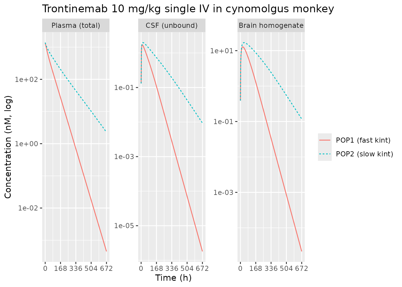
Trontinemab 10 mg/kg in NHP: simulated plasma total drug (Cc), CSF unbound (Ccsf), and whole-brain homogenate (Cbrain) concentrations vs. time. POP1/POP2 are the two kint subpopulations from the mixture model. Replicates Figure 3 trontinemab panel of Muliaditan 2025.
Simulation 2 – non-TfR control mAb in NHP (sanity check)
Setting kon_T = 0 (encoded as a tiny placeholder
1e-12 in ini()) collapses all TfR-mediated
dynamics. The simulated profiles should look like a generic linear-PK
mAb in plasma with very low brain / CSF exposure (the FAC_BPRED = 0.05
brain-correction factor scales the brain prediction downward by 20-fold
relative to the brain ISF concentration).
sim_control <- rxode2::rxSolve(
  mod_nhp_typ,
  events = ev_nhp,
  params = c(MIX_FAST_ELIM = 0,
             # Default ini() already encodes non-TfR control; show parameters
             # explicitly here for clarity.
             lkon_t  = log(1e-12),
             lkoff_t = log(1),
             mw_kda  = 150)   # generic IgG
) |> as.data.frame()

control_summary <- sim_control |>
  filter(time > 0) |>
  summarise(Cc_max = max(Cc), Ccsf_max = max(Ccsf), Cbrain_max = max(Cbrain))
knitr::kable(control_summary,
caption = "Peak concentrations for a non-TfR control mAb at 10 mg/kg in NHP")| Cc_max | Ccsf_max | Cbrain_max |
|---|---|---|
| 1195.233 | 1.924228 | 0.4767569 |
The brain and CSF peaks for the non-TfR control are much lower than the corresponding peaks for trontinemab (Simulation 1) – consistent with the paper’s observation that anti-TfR bsAbs achieve enhanced brain delivery relative to non-binders.
Simulation 3 – trontinemab in human, single ascending doses (replicates Figure 5)
mod_hum <- nlmixr2lib::readModelDb("Muliaditan_2025_mab_mpbpk_human")
mod_hum_typ <- rxode2::zeroRe(mod_hum)
#> Warning: No omega parameters in the model

human_doses_mgkg <- c(0.1, 0.4, 1.2, 3.6, 7.2)
human_doses_mg   <- human_doses_mgkg * human_wt_kg

times_h <- seq(0.5, 168, length.out = 120)

build_human_events <- function(dose_mg, id_offset) {
  rxode2::et(time = 0, amt = dose_mg, cmt = "central") |>
    rxode2::et(times_h, cmt = "Cc") |>
    as.data.frame() |>
    mutate(id = id_offset + 1L,
           dose_mgkg = dose_mg / human_wt_kg)
}

events_human <- purrr::map2_dfr(
  human_doses_mg, seq_along(human_doses_mg) - 1L,
  build_human_events
)

sim_human <- rxode2::rxSolve(
  mod_hum_typ,
  events = events_human,
  params = c(MIX_FAST_ELIM = 0,
             lkon_t  = log(tron_hum_kon),
             lkoff_t = log(tron_hum_koff),
             mw_kda  = trontinemab_mw),
  keep = "dose_mgkg"
) |> as.data.frame()
#> Warning: multi-subject simulation without without 'omega'
sim_human_plot <- sim_human |>
  filter(time > 0) |>
  pivot_longer(c(Cc, Ccsf), names_to = "Matrix", values_to = "Conc_nM") |>
  mutate(dose_label = sprintf("%.1f mg/kg", dose_mgkg))

ggplot(sim_human_plot, aes(time, pmax(Conc_nM, 1e-6), colour = dose_label)) +
  geom_line() +
  facet_wrap(~ factor(Matrix, levels = c("Cc", "Ccsf"),
                       labels = c("Plasma (total)", "CSF (unbound)")),
             scales = "free_y") +
  scale_y_log10() +
  labs(x = "Time (h)", y = "Concentration (nM, log)",
       colour = "Dose",
       title = "Trontinemab single ascending dose in human")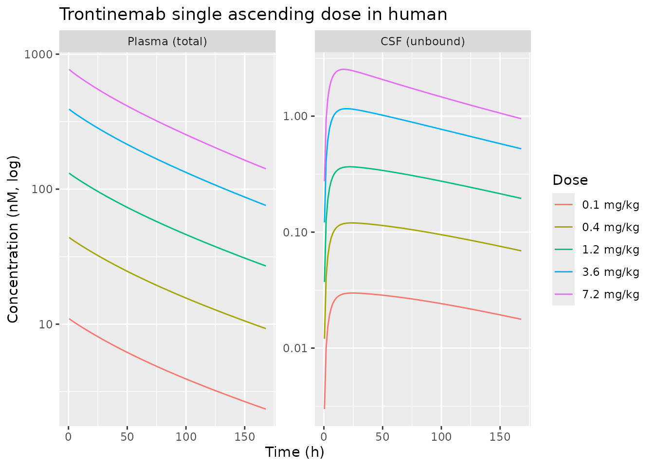
Trontinemab single ascending IV doses (0.1-7.2 mg/kg) in healthy adult subjects: simulated plasma total drug Cc and CSF unbound Ccsf vs. time. Replicates Figure 5 of Muliaditan 2025.
Simulation 4 – predicted brain AUC vs TfR binding affinity (replicates Figure 4)
The paper’s Figure 4 sweeps KD,TfR from 0 to 3000 nM in
NHP at single ascending doses 1-100 mg/kg and shows that dose-normalised
brain AUC0-672h peaks in the 800-3000 nM range. This block
reproduces the qualitative shape at a single 10 mg/kg dose.
kd_grid <- c(0, 30, 100, 300, 1000, 3000)   # nM
# Use the paper's average per-compound kon_T = 0.5193 nM^-1 h^-1, then
# derive koff_T from koff = KD * kon.
kon_T_typical <- 0.5193

sweep_brain_auc <- function(kd_nM) {
  if (kd_nM == 0) {
    kon  <- 1e-12
    koff <- 1
  } else {
    kon  <- kon_T_typical
    koff <- kd_nM * kon_T_typical
  }
  sim <- rxode2::rxSolve(
    mod_nhp_typ,
    events = rxode2::et(time = 0, amt = nhp_dose_mg, cmt = "central") |>
              rxode2::et(seq(2, 672, length.out = 120), cmt = "Cbrain"),
    params = c(MIX_FAST_ELIM = 0,
               lkon_t  = log(kon),
               lkoff_t = log(koff),
               mw_kda  = trontinemab_mw)
  ) |> as.data.frame()
  # Trapezoidal AUC over 0-672 h for brain homogenate concentration
  sim <- sim |> filter(!is.na(Cbrain)) |> arrange(time)
  auc <- sum(diff(sim$time) * (head(sim$Cbrain, -1) + tail(sim$Cbrain, -1)) / 2)
  data.frame(KD_nM = kd_nM, brain_AUC_nMh = auc)
}

kd_sweep <- purrr::map_dfr(kd_grid, sweep_brain_auc)
knitr::kable(kd_sweep, caption = "Brain AUC0-672h vs TfR KD (10 mg/kg NHP)")| KD_nM | brain_AUC_nMh |
|---|---|
| 0 | 149.3032 |
| 30 | 949.3885 |
| 100 | 2135.2927 |
| 300 | 3678.1496 |
| 1000 | 5024.8554 |
| 3000 | 4125.2488 |
control_auc <- kd_sweep$brain_AUC_nMh[kd_sweep$KD_nM == 0]
ggplot(kd_sweep |> filter(KD_nM > 0),
       aes(KD_nM, brain_AUC_nMh)) +
  geom_line() +
  geom_point() +
  geom_hline(yintercept = control_auc, linetype = "dashed") +
  scale_x_log10() +
  labs(x = "KD,TfR (nM, log)",
       y = "Brain AUC0-672h (nM*h)",
       title = "Brain AUC vs TfR binding affinity in NHP")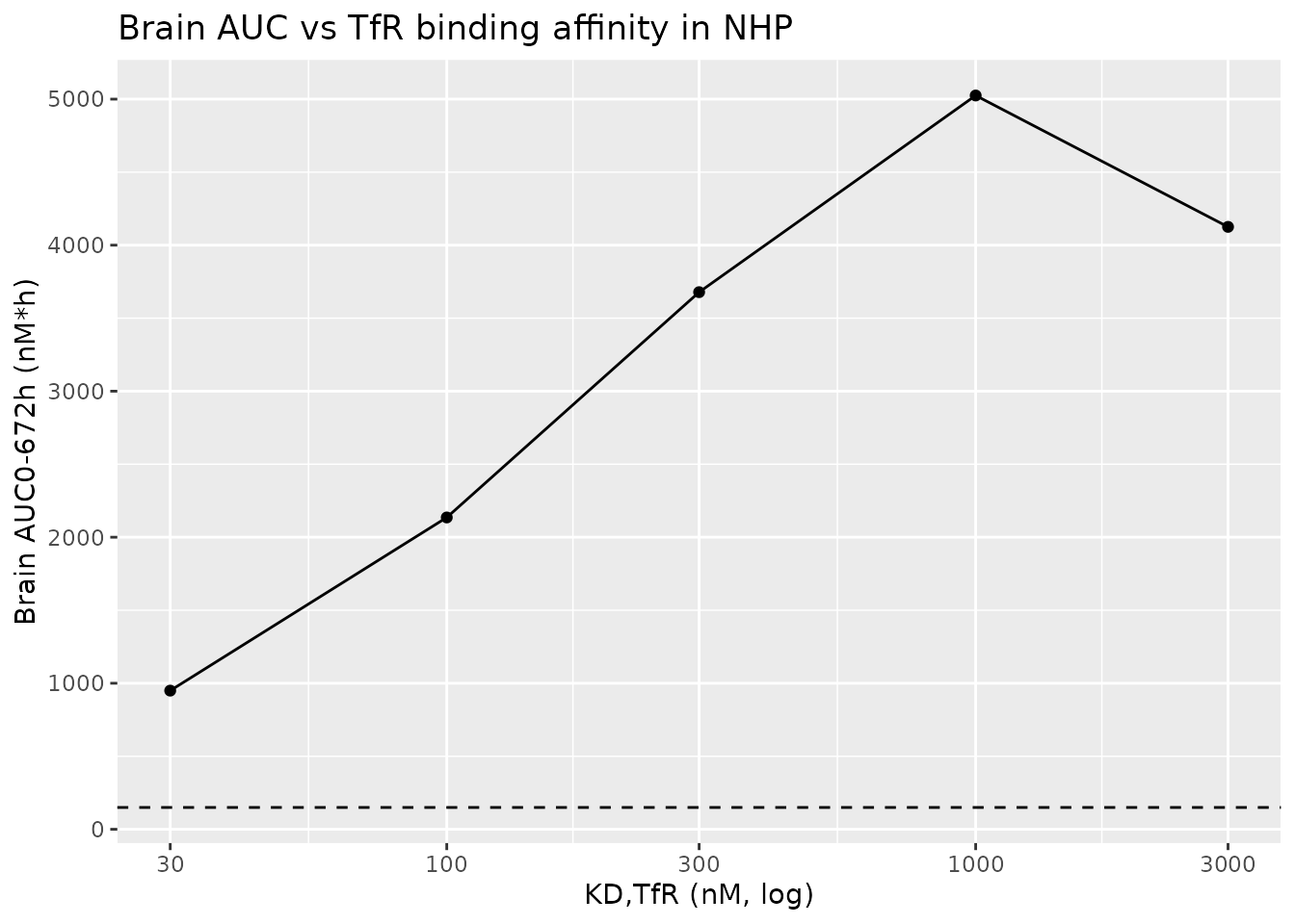
Dose-normalised brain AUC0-672h vs TfR binding affinity in NHP at 10 mg/kg. Horizontal dashed line is the non-TfR control mAb. Replicates the qualitative finding of Figure 4 of Muliaditan 2025.
PKNCA validation – human trontinemab plasma exposure
PKNCA is applied to plasma total drug Cc from Simulation
3 to compute Cmax, Tmax, AUC0-168h, AUC0-inf, and half-life per dose
group, then compared against the published metrics in Muliaditan 2025
Figure 5c. The paper reports observed plasma AUC0-168h, AUC0-inf, and
Cmax from the trontinemab Phase 1 trial (NCT04023994). Because the paper
only shows these graphically (no per-dose tabulated table in the main
text), the comparison here is qualitative.
sim_human_nca <- sim_human |>
  dplyr::filter(!is.na(Cc)) |>
  dplyr::select(id, time, Cc, dose_mgkg) |>
  dplyr::mutate(treatment = sprintf("%.1f mg/kg", dose_mgkg))

# Guarantee a time-zero row per (id, treatment); for IV bolus pre-dose Cc = 0.
sim_human_nca <- dplyr::bind_rows(
  sim_human_nca,
  sim_human_nca |> dplyr::distinct(id, treatment, dose_mgkg) |>
    dplyr::mutate(time = 0, Cc = 0)
) |>
  dplyr::distinct(id, treatment, time, .keep_all = TRUE) |>
  dplyr::arrange(id, treatment, time)

conc_obj <- PKNCA::PKNCAconc(sim_human_nca, Cc ~ time | treatment + id)

dose_df <- events_human |>
  dplyr::filter(evid == 1) |>
  dplyr::mutate(treatment = sprintf("%.1f mg/kg", dose_mgkg)) |>
  dplyr::select(id, time, amt, treatment)

dose_obj <- PKNCA::PKNCAdose(dose_df, amt ~ time | treatment + id)

intervals <- data.frame(
  start       = 0,
  end         = 168,
  cmax        = TRUE,
  tmax        = TRUE,
  auclast     = TRUE,
  aucinf.obs  = TRUE,
  half.life   = TRUE
)

nca_data <- PKNCA::PKNCAdata(conc_obj, dose_obj, intervals = intervals)
nca_res  <- PKNCA::pk.nca(nca_data)

nca_tbl <- as.data.frame(nca_res$result) |>
  select(treatment, PPTESTCD, PPORRES) |>
  pivot_wider(names_from = PPTESTCD, values_from = PPORRES)

knitr::kable(nca_tbl,
caption = "Simulated trontinemab plasma NCA per dose group (nM, nM*h, h)")| treatment | auclast | cmax | tmax | tlast | clast.obs | lambda.z | r.squared | adj.r.squared | lambda.z.time.first | lambda.z.time.last | lambda.z.n.points | clast.pred | half.life | span.ratio | aucinf.obs |
|---|---|---|---|---|---|---|---|---|---|---|---|---|---|---|---|
| 0.1 mg/kg | 863.800 | 10.98751 | 0.5 | 168 | 2.348425 | 0.0072585 | 0.9999107 | 0.9999068 | 134.2185 | 168 | 25 | 2.345282 | 95.49467 | 0.3537528 | 1187.342 |
| 0.4 mg/kg | 3439.817 | 43.91784 | 0.5 | 168 | 9.269410 | 0.0073760 | 0.9999059 | 0.9999020 | 132.8109 | 168 | 26 | 9.255869 | 93.97393 | 0.3744557 | 4696.524 |
| 1.2 mg/kg | 10207.035 | 131.48215 | 0.5 | 168 | 26.983444 | 0.0076107 | 0.9999057 | 0.9999019 | 131.4034 | 168 | 27 | 26.940816 | 91.07506 | 0.4018294 | 13752.486 |
| 3.6 mg/kg | 29752.623 | 391.59372 | 0.5 | 168 | 75.808999 | 0.0080382 | 0.9999071 | 0.9999037 | 128.5882 | 168 | 29 | 75.672376 | 86.23195 | 0.4570437 | 39183.748 |
| 7.2 mg/kg | 57218.906 | 771.68380 | 0.5 | 168 | 141.491969 | 0.0083788 | 0.9999043 | 0.9999011 | 124.3655 | 168 | 32 | 141.190457 | 82.72621 | 0.5274562 | 74105.788 |
Assumptions and deviations
-
Brain homogenate equation simplification. The
supplement equation for
CBrHomo0includes a contribution from ventricular CSFA(12) * (VCSFLV + VCSFTFV)and a denominator(VBtotal + VCSFLV + VCSFTFV). The volumesVBtotal,VCSFLV, andVCSFTFVare Bloomingdale 2017 model constants that are not reported in the Muliaditan 2025 paper, supplement, or any other on-disk source for this extraction. The model file therefore approximatesCbrainas a volume-weighted average over the (BBB endosomal + brain ISF + BCSFB endosomal) compartments only, scaled by the estimatedFAC_BPRED = 0.05correction. This is a strict subset of the published equation and may under-predict brain homogenate by a small amount that depends on ventricular CSF contribution. Users who want the full equation can re-deriveVBtotal,VCSFLV, andVCSFTFVfrom the Bloomingdale 2017 source publication and pass them through a wrapper that recomputesCbrainpost hoc from the rxode2 state vector. -
Mixture model selection. The paper’s NONMEM mixture
model assigns each subject to either POP1 (fast kint, fraction 0.437) or
POP2 (slow kint, fraction 0.563) without correlation to KD,TfR or data
source. The model file exposes this as the canonical binary covariate
MIX_FAST_ELIM. Typical-value simulation usesMIX_FAST_ELIM = 0(slow, dominant subpopulation); population simulations should drawMIX_FAST_ELIM ~ Bernoulli(0.437)per subject. -
No inter-individual variability. The paper did not
estimate IIV because the NHP dataset was largely mean digitised
profiles. The model files therefore carry no
eta*parameters;rxode2::zeroRe()is cosmetic on these models since there is nothing to zero. -
Per-compound TfR binding inputs.
kon_Tandkoff_Tare NOT population estimates - they are biophysical inputs taken from each compound’s binding assay (paper Table S2). The defaultini()encodes a non-TfR control IgG (kon_T = 1e-12placeholder). To simulate a specific antibody, overridelkon_t,lkoff_t, andmw_kdavia theparams =argument torxSolve(). -
Plasma observation is TOTAL drug. Per paper
Methods, plasma measurements are total drug (free + TfR-bound complex).
The model file observation
Cc <- c_plasma + c_complex_plasmamatches this; CSF and brain observations are unbound / homogenate concentrations respectively. -
Allometric scaling between NHP and human. Both
kint POP1andkint POP2are scaled from NHP to human by(70/6.2)^(-0.25) = 0.546per the paper’s stated exponent. The paper explicitly reports the POP1 scaling (0.0329 -> 0.0179) but does not tabulate the POP2 scaling; the human file applies the same allometric formula to POP2 (0.0125 -> 0.00683). -
Synthesis rates for luminal BBB / BCSFB TfR.
Ksyn_uTfRBBBandKsyn_uTfRBCSFBare not reported as separate parameters in the paper. At steady state without drug they are constrained by the baseline:Ksyn = Kdeg * uTFR0. The model file derives them inline fromKdeg_uTfRanduTFR0per this steady-state identity. -
FcRn baseline initial conditions. The supplement
states “The initial condition for all the compartments is 0, except for
unbound FcRn (A14-A16)”. The model file initialises the free-FcRn
compartments at
FcRn * V(whereFcRn = 4.98e-5 mol/Lfrom Supp Table S1).