Brepocitinib (Tsamandouras 2024)
Source:vignettes/articles/Tsamandouras_2024_brepocitinib.Rmd
Tsamandouras_2024_brepocitinib.RmdModel and source
- Citation: Tsamandouras N, Qiu R, Hughes JH, Sweeney K, Prybylski JP, Banfield C, Nicholas T. Employing zero-inflated beta distribution in an exposure-response analysis of TYK2/JAK1 inhibitor brepocitinib in patients with plaque psoriasis. J Pharmacokinet Pharmacodyn. 2024;51(3):265-277. doi:10.1007/s10928-024-09901-2. The CAV input comes from the brepocitinib population PK model of Hughes JH et al. Clin Pharmacol Drug Dev. 2022;11(12):1447-1456. doi:10.1002/cpdd.1163; see modellib(‘Hughes_2022_brepocitinib’).
- Description: Exposure-response model for the Psoriasis Area and Severity Index (PASI) under oral brepocitinib (PF-06700841, a dual TYK2/JAK1 inhibitor) in adults with moderate-to-severe plaque psoriasis (Tsamandouras 2024). The PASI score divided by 72 follows a zero-inflated beta distribution: a point mass at PASI = 0 whose logit falls linearly with the beta mean, and a beta density with mean mu and precision phi otherwise. The expected score is the baseline (logit-normal between 12 and 72) minus an exponential placebo effect that removes at most a fraction Pmax of baseline, minus a drug effect on the remaining fraction driven by a type I indirect-response latent variable whose production the individual average steady-state brepocitinib concentration (CAV) inhibits.
- Article: https://doi.org/10.1007/s10928-024-09901-2 (open access, PMC11136736)
- Supplement: Online Resource 1 of the article (NONMEM control stream
run6.mod)
Tsamandouras et al. analysed the Psoriasis Area and Severity Index
(PASI) from the phase 2a study of brepocitinib in plaque psoriasis
(NCT02969018). The PASI score divided by 72 was modelled with a
zero-inflated beta distribution: a point mass at PASI = 0 and a beta
density on (0, 1) whose mean mu is the model-predicted
score. The expected score falls from an individual baseline through an
exponential placebo effect and a drug effect delivered through a type I
indirect-response latent variable R(t), whose production
the individual average steady-state brepocitinib concentration
CAV inhibits.
Population
212 adults with moderate-to-severe plaque psoriasis (PASI >= 12, PGA 3 or 4, >= 10% body surface area involved) were randomized to eight arms: a 4-week induction period with brepocitinib 30 or 60 mg once daily (QD) or placebo, then an 8-week maintenance period with 10 or 30 mg QD, 100 mg once weekly (QW) or placebo (Table 1 and Figure 1 of the paper). The participants were 69.8% male and 89.2% White, with median age 48 years (18-75), median weight 91.6 kg (45.1-204.3) and median baseline PASI 18.2 (12-54). Only PASI scores from weeks 0-12 were analysed, and no covariates were tested.
The same information is available programmatically via
readModelDb("Tsamandouras_2024_brepocitinib")()$population.
Source trace
Every ini() value carries an in-file comment pointing to
its source. The table collects them, together with the equations.
| Equation / parameter | Value | Source location |
|---|---|---|
logitrbase (BSL) |
logit((18.00 - 12) / 60) | Table 2 BSL = 18.00; Eq. 14 with bounds 12 and 72 |
imax |
1 (fixed) | Online Resource 1 $THETA ‘1 FIX ; IMAX’ |
lic50 (IC50) |
log(53.24) ng/mL | Table 2 |
lkout (kout = kin) |
log(0.067) 1/day | Table 2 and its footnote |
logitpmax (Pmax) |
logit(0.489) | Table 2; Online Resource 1 LGPMAX
|
lkpbo (kp) |
log(0.047) 1/day | Table 2 |
lphi (phi) |
log(31.25) | Table 2 |
logite0_pasi0 (zeta1) |
2.228 | Table 2 |
e_mu_pasi0 (zeta2) |
62.67 | Table 2 |
etalogitrbase |
1.655 | Table 2 ‘etaBSL omega2’ |
Average concentration CAV = Dose / (CL/F * tau)
|
– | Eq. 1 |
Transformed score y = PASI / 72
|
– | Eq. 2 |
| Zero-inflated beta density | – | Eq. 3-4 |
| Nemes approximation to the gamma function | – | Eq. 5; Online Resource 1 LGAMMAX1-3
|
alpha = mu * phi,
beta = (1 - mu) * phi
|
– | Eq. 6-7 |
mu = (BSL - fp(t) - fd(t)) / 72 |
– | Eq. 9 |
fp(t) = BSL * Pmax * (1 - exp(-kp * t)) |
– | Eq. 10 |
fd(t) = BSL * (1 - Pmax) * (1 - R(t)) |
– | Eq. 11 |
dR/dt = kin * (1 - CAV / (IC50 + CAV)) - kout * R,
R(0) = 1
|
– | Eq. 12 |
p0 = expit(zeta1 - zeta2 * mu) |
– | Eq. 13 |
| Logit-normal IIV on the baseline, bounds 12 and 72 | – | Eq. 14; Online Resource 1 LGBASE
|
Exposure input: CAV from the Hughes 2022 population PK model
The paper derives each participant’s CAV from the
empirical Bayes CL/F of the brepocitinib population PK model of Hughes
et al. (2022), shipped as
modellib("Hughes_2022_brepocitinib"): CL/F = 18.7 L/h at 70
kg, a fixed weight exponent of 0.75 and 78% CV. Its clinical trial
simulations sample CL/F from that distribution after applying each
simulated participant’s weight. The code below does the same, taking the
typical value, exponent and variance from the shipped PK model.
pk <- rxode2::rxode2(readModelDb("Hughes_2022_brepocitinib"))
cl_typ <- exp(pk$theta[["lcl"]])
e_wt_cl <- pk$theta[["e_wt_cl"]]
omega_cl <- pk$omega["etalcl", "etalcl"]
c(cl_typ = cl_typ, e_wt_cl = e_wt_cl, omega_cl = omega_cl)
#>   cl_typ  e_wt_cl omega_cl
#>  18.7000   0.7500   0.6084

# Dose in mg, CL/F in L/h, tau in h; x 1000 gives ng/mL (Eq. 1).
cav_ngml <- function(dose_mg, cl_lh, tau_h) dose_mg * 1000 / (cl_lh * tau_h)
Virtual cohort
The paper sampled weights with replacement from the study dataset,
which is not public. The cohort here draws log-normal weights around the
reported median of 91.6 kg, truncated to the observed 45.1-204.3 kg
range. All random numbers come from base R after
set.seed(), and the between-subject random effects are
passed to rxSolve() through params, so the
cohort does not depend on the rxode2 build or thread count. The same 200
participants are used in every arm, which makes the arm comparisons
paired.
set.seed(20240302)
n_per_arm <- 200
mod <- rxode2::rxode2(readModelDb("Tsamandouras_2024_brepocitinib"))
#> ℹ parameter labels from comments will be replaced by 'label()'

cohort <- data.frame(id = seq_len(n_per_arm)) |>
  mutate(
    WT = pmin(pmax(exp(rnorm(n(), log(91.6), 0.22)), 45.1), 204.3),
    cl = cl_typ * (WT / 70)^e_wt_cl * exp(rnorm(n(), 0, sqrt(omega_cl))),
    etalogitrbase = rnorm(n(), 0, sqrt(mod$omega["etalogitrbase", "etalogitrbase"]))
  )
summary(cohort$WT)
#>    Min. 1st Qu.  Median    Mean 3rd Qu.    Max.
#>   53.07   75.45   90.06   92.82  105.61  164.68
The observation step draws the score from the zero-inflated beta
distribution: PASI = 0 with probability p0_pasi, otherwise
72 * Beta(alpha_pasi, beta_pasi).
# Simulate one regimen in the cohort. `ind` and `maint` are the regimens of the
# induction (days 0-27) and maintenance (day 28 on) periods: dose in mg and
# dosing interval in h (24 for QD, 168 for QW); dose 0 is placebo.
sim_regimen <- function(label, ind, maint, times) {
  cav_ind <- cav_ngml(ind$dose, cohort$cl, ind$tau)
  cav_maint <- cav_ngml(maint$dose, cohort$cl, maint$tau)
  events <- tidyr::expand_grid(id = cohort$id, time = times) |>
    mutate(
      evid = 0L,
      amt = 0,
      # CAV is carried forward from each row, so the value on the day-28 row
      # is the maintenance exposure from day 28 onwards.
      CAV = ifelse(time < 28, cav_ind[id], cav_maint[id])
    )
  sim <- rxode2::rxSolve(
    rxode2::zeroRe(mod),
    events = events,
    params = cohort[, c("id", "etalogitrbase")],
    covsInterpolation = "locf",
    returnType = "data.frame"
  )
  sim$regimen <- label
  sim$CAV <- events$CAV
  sim
}

draw_pasi <- function(sim) {
  zero <- runif(nrow(sim)) < sim$p0_pasi
  sim$pasi <- ifelse(zero, 0, 72 * rbeta(nrow(sim), sim$alpha_pasi, sim$beta_pasi))
  sim
}

responders <- function(sim) {
  base <- sim |>
    filter(time == 0) |>
    select(regimen, id, pasi_bl = pasi)
  sim |>
    inner_join(base, by = c("regimen", "id")) |>
    mutate(pct_imp = 100 * (1 - pasi / pasi_bl)) |>
    group_by(regimen, time) |>
    summarise(
      PASI50 = 100 * mean(pct_imp >= 50),
      PASI75 = 100 * mean(pct_imp >= 75),
      PASI90 = 100 * mean(pct_imp >= 90),
      PASI100 = 100 * mean(pct_imp >= 100),
      .groups = "drop"
    )
}

qd <- function(dose) list(dose = dose, tau = 24)
qw <- function(dose) list(dose = dose, tau = 168)
Likelihood check
ll(pasi) encodes the zero-inflated beta log-likelihood
exactly as the paper’s control stream does, including the Nemes
approximation to the log gamma function. Solving the model with a
DV column and comparing against a closed form computed in R
from the same mu, phi and p0
confirms the encoding.
nemes <- function(x) {
  x * (log(x) - 1) + 0.5 * (log(2 * 3.1415) - log(x)) +
    1.25 * x * log(1 + 1 / (15 * x^2))
}
ll_events <- data.frame(
  id = 1L,
  time = c(0, 14, 28, 56, 84, 84),
  evid = 0L,
  amt = 0,
  CAV = 54.5,
  DV = c(18, 12.3, 0, 4.2, 0.6, 0)
)
ll_sim <- rxode2::rxSolve(rxode2::zeroRe(mod), events = ll_events, returnType = "data.frame")
#> Warning: No sigma parameters in the model
#> ℹ omega/sigma items treated as zero: 'etalogitrbase'
ll_ref <- with(ll_sim, ifelse(
  DV == 0,
  log(p0_pasi),
  nemes(phi) - nemes(alpha_pasi) - nemes(beta_pasi) +
    (alpha_pasi - 1) * log(DV / 72) + (beta_pasi - 1) * log(1 - DV / 72) +
    log(1 - p0_pasi)
))
ll_exact <- with(ll_sim, ifelse(
  DV == 0,
  log(p0_pasi),
  dbeta(DV / 72, alpha_pasi, beta_pasi, log = TRUE) + log(1 - p0_pasi)
))
ll_sim |>
  mutate(ll_closed_form = ll_ref, ll_exact_gamma = ll_exact) |>
  select(time, DV, mu_pasi, p0_pasi, ll_pasi, ll_closed_form, ll_exact_gamma) |>
knitr::kable(digits = 5)| time | DV | mu_pasi | p0_pasi | ll_pasi | ll_closed_form | ll_exact_gamma |
|---|---|---|---|---|---|---|
| 0 | 18.0 | 0.25000 | 0.00000 | 1.62752 | 1.62752 | 1.62751 |
| 14 | 12.3 | 0.15173 | 0.00069 | 1.67117 | 1.67117 | 1.67115 |
| 28 | 0.0 | 0.10582 | 0.01209 | -4.41568 | -4.41568 | -4.41568 |
| 56 | 4.2 | 0.07344 | 0.08515 | 2.17446 | 2.17446 | 2.17443 |
| 84 | 0.6 | 0.06572 | 0.13118 | 1.52091 | 1.52091 | 1.52088 |
| 84 | 0.0 | 0.06572 | 0.13118 | -2.03122 | -2.03122 | -2.03122 |
# The model's ll and the R closed form use the same inputs, so they must agree
# to floating-point precision.
stopifnot(max(abs(ll_sim$ll_pasi - ll_ref)) < 1e-8)
The last column replaces the Nemes approximation with the exact log gamma function. The two agree closely while the beta shapes are above 1, and the approximation drifts when a shape falls well below 1 (a predicted score of a few tenths of a point); the parameter estimates were obtained with the approximation, so the model keeps it.
Clinical trial simulation: week-16 responder rates (Figure 5)
The paper simulated placebo and brepocitinib 5-60 mg QD for 16 weeks with 56 participants per arm and 2000 trials, assessing PASI at baseline and every 2 weeks. One trial of 200 participants per arm is simulated here for placebo, 10, 30 and 60 mg QD.
times_16 <- seq(0, 112, by = 14)
flat_doses <- c(0, 10, 30, 60)
sim16 <- bind_rows(lapply(flat_doses, function(d) {
  lbl <- if (d == 0) "Placebo QD" else paste(d, "mg QD")
  sim_regimen(lbl, qd(d), qd(d), times_16)
})) |>
  draw_pasi()
#> Warning: No sigma parameters in the model
#> No sigma parameters in the model
#> No sigma parameters in the model
#> No sigma parameters in the model

resp16 <- responders(sim16) |>
  filter(time == 112)

cav_med <- sim16 |>
  filter(time == 0) |>
  group_by(regimen) |>
  summarise(sim = median(CAV), .groups = "drop")
The median CAV matches the values in the bottom panels
of Figure 5:
cav_cmp <- data.frame(
  regimen = c("10 mg QD", "30 mg QD", "60 mg QD"),
  paper = c(18.1, 54.5, 108.6)
) |>
  inner_join(cav_med, by = "regimen") |>
  mutate(pct_diff = 100 * (sim - paper) / paper)
cav_cmp |>
  rename(
    Regimen = regimen,
    "Paper median CAV (ng/mL)" = paper,
    "Simulated median CAV (ng/mL)" = sim,
    "Difference (%)" = pct_diff
  ) |>
knitr::kable(digits = 1)| Regimen | Paper median CAV (ng/mL) | Simulated median CAV (ng/mL) | Difference (%) |
|---|---|---|---|
| 10 mg QD | 18.1 | 17.0 | -6.2 |
| 30 mg QD | 54.5 | 50.9 | -6.6 |
| 60 mg QD | 108.6 | 101.8 | -6.2 |
# The median CAV is set by the typical CL/F at the 91.6 kg median weight; a
# wrong CL/F, weight exponent or unit conversion moves it by far more.
stopifnot(all(abs(cav_cmp$pct_diff) < 15))
The week-16 responder rates against the medians printed on Figure 5:
paper16 <- data.frame(
  regimen = rep(c("Placebo QD", "10 mg QD", "30 mg QD", "60 mg QD"), each = 3),
  metric = rep(c("PASI75", "PASI90", "PASI100"), 4),
  paper = c(
    12.5, 1.8, 0.0,
    35.7, 12.5, 5.4,
    62.5, 35.7, 21.4,
    78.6, 55.4, 35.7
  )
)
cmp16 <- resp16 |>
  pivot_longer(c(PASI75, PASI90, PASI100), names_to = "metric", values_to = "sim") |>
  inner_join(paper16, by = c("regimen", "metric")) |>
  mutate(diff = sim - paper) |>
  arrange(match(regimen, unique(paper16$regimen)), match(metric, c("PASI75", "PASI90", "PASI100")))
cmp16 |>
  select(regimen, metric, paper, sim, diff) |>
  rename(
    Regimen = regimen,
    Metric = metric,
    "Paper, week 16 (%)" = paper,
    "Simulated, week 16 (%)" = sim,
    "Difference (percentage points)" = diff
  ) |>
knitr::kable(digits = 1)| Regimen | Metric | Paper, week 16 (%) | Simulated, week 16 (%) | Difference (percentage points) |
|---|---|---|---|---|
| Placebo QD | PASI75 | 12.5 | 12.0 | -0.5 |
| Placebo QD | PASI90 | 1.8 | 2.5 | 0.7 |
| Placebo QD | PASI100 | 0.0 | 1.5 | 1.5 |
| 10 mg QD | PASI75 | 35.7 | 34.0 | -1.7 |
| 10 mg QD | PASI90 | 12.5 | 9.5 | -3.0 |
| 10 mg QD | PASI100 | 5.4 | 4.5 | -0.9 |
| 30 mg QD | PASI75 | 62.5 | 63.0 | 0.5 |
| 30 mg QD | PASI90 | 35.7 | 28.5 | -7.2 |
| 30 mg QD | PASI100 | 21.4 | 17.0 | -4.4 |
| 60 mg QD | PASI75 | 78.6 | 82.0 | 3.4 |
| 60 mg QD | PASI90 | 55.4 | 59.5 | 4.1 |
| 60 mg QD | PASI100 | 35.7 | 40.0 | 4.3 |
stopifnot(
  # A mis-transcribed IC50, kout, Pmax or zeta moves every arm by well over
  # this; one 200-subject trial has a binomial SE of about 3.5 points.
  abs(median(cmp16$diff)) < 5,
  quantile(abs(cmp16$diff), 0.9) < 10
)
cmp16 |>
  mutate(
    dose = c("Placebo QD" = 0, "10 mg QD" = 10, "30 mg QD" = 30, "60 mg QD" = 60)[regimen],
    metric = factor(metric, levels = c("PASI75", "PASI90", "PASI100"))
  ) |>
  ggplot(aes(dose)) +
  geom_line(aes(y = sim)) +
  geom_point(aes(y = sim)) +
  geom_point(aes(y = paper), shape = 4, size = 3, colour = "darkorange") +
  facet_wrap(~metric) +
  labs(x = "Dose (mg QD)", y = "Responders at week 16 (%)") +
  theme_bw()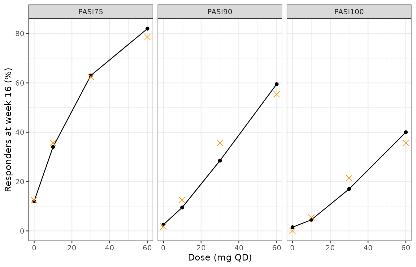
Replicates the top panels of Figure 5 of Tsamandouras 2024 for placebo, 10, 30 and 60 mg QD: week-16 responder rates (points: this simulation; crosses: medians printed on the paper’s figure).
Flat dosing versus induction and maintenance (Figure 6)
The paper compared 10, 30 and 60 mg QD for 16 weeks against 60 mg QD for 4 weeks followed by 10 or 30 mg QD for 12 weeks, and found that the induction-maintenance regimens converge to the matching flat dose by week 16.
sim_im <- bind_rows(
  sim_regimen("60 mg QD / 10 mg QD", qd(60), qd(10), times_16),
  sim_regimen("60 mg QD / 30 mg QD", qd(60), qd(30), times_16)
) |>
  draw_pasi()
#> Warning: No sigma parameters in the model
#> No sigma parameters in the model
sim6 <- bind_rows(filter(sim16, regimen != "Placebo QD"), sim_im)

pasi6 <- sim6 |>
  group_by(regimen, time) |>
  summarise(median_pasi = median(pasi), .groups = "drop")
resp6 <- responders(sim6)
bind_rows(
  pasi6 |> transmute(regimen, time, panel = "Median PASI", value = median_pasi),
  resp6 |>
    pivot_longer(c(PASI75, PASI90, PASI100), names_to = "panel") |>
    select(regimen, time, panel, value)
) |>
  mutate(panel = factor(panel, levels = c("Median PASI", "PASI75", "PASI90", "PASI100"))) |>
  ggplot(aes(time / 7, value, colour = regimen)) +
  geom_line() +
  geom_point(size = 1) +
  facet_wrap(~panel, scales = "free_y") +
  labs(x = "Week", y = NULL, colour = NULL) +
  theme_bw() +
  theme(legend.position = "bottom")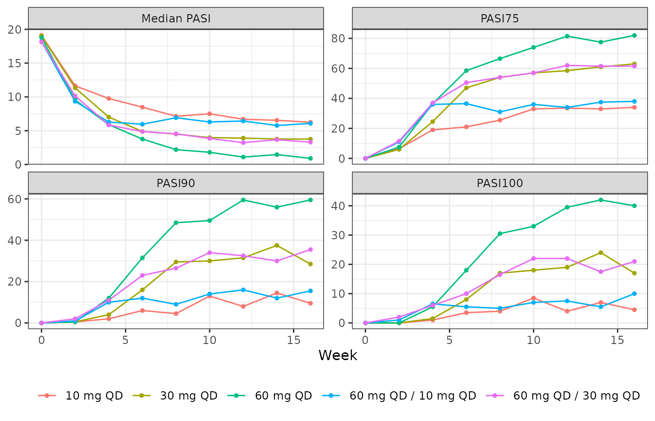
Replicates Figure 6 of Tsamandouras 2024: median PASI and PASI75/90/100 responder rates over 16 weeks for flat dosing and for 4 weeks of 60 mg QD induction followed by 10 or 30 mg QD.
Because the cohorts are paired, the mean of the individual predicted scores (before the zero-inflated beta draw) isolates the regimen effect. With kout = 0.067/day the latent variable re-equilibrates with a half-life of about 10 days, so 12 weeks of maintenance erase the induction:
typ <- sim6 |>
  filter(time == 112) |>
  group_by(regimen) |>
  summarise(mean_pasi_pred = mean(pasi_pred), .groups = "drop")
typ |>
  rename(Regimen = regimen, "Mean predicted PASI at week 16" = mean_pasi_pred) |>
knitr::kable(digits = 3)| Regimen | Mean predicted PASI at week 16 |
|---|---|
| 10 mg QD | 7.718 |
| 30 mg QD | 5.377 |
| 60 mg QD | 3.823 |
| 60 mg QD / 10 mg QD | 7.706 |
| 60 mg QD / 30 mg QD | 5.372 |
conv <- with(typ, c(
  ten = mean_pasi_pred[regimen == "60 mg QD / 10 mg QD"] / mean_pasi_pred[regimen == "10 mg QD"] - 1,
  thirty = mean_pasi_pred[regimen == "60 mg QD / 30 mg QD"] / mean_pasi_pred[regimen == "30 mg QD"] - 1
))
conv
#>           ten        thirty
#> -0.0015376712 -0.0008804797
# Same participants and parameters in both regimens, so the difference is the
# residual induction effect alone: exp(-0.067 * 84) is about 0.4%.
stopifnot(all(abs(conv) < 0.01))
Study-design simulation (Figures 3 and 4)
The eight arms of the phase 2a study, with the induction regimen up to week 4 and the maintenance regimen from week 5 to week 12, simulated at the study’s assessment weeks (0, 1, 2, 4, 6, 8, 10 and 12).
times_12 <- c(0, 1, 2, 4, 6, 8, 10, 12) * 7
arms <- list(
  list("Placebo QD", qd(0), qd(0)),
  list("30 mg QD / 10 mg QD", qd(30), qd(10)),
  list("30 mg QD / 100 mg QW", qd(30), qw(100)),
  list("30 mg QD", qd(30), qd(30)),
  list("60 mg QD / Placebo QD", qd(60), qd(0)),
  list("60 mg QD / 10 mg QD", qd(60), qd(10)),
  list("60 mg QD / 100 mg QW", qd(60), qw(100)),
  list("60 mg QD / 30 mg QD", qd(60), qd(30))
)
arm_levels <- vapply(arms, `[[`, character(1), 1)
sim12 <- bind_rows(lapply(arms, function(a) sim_regimen(a[[1]], a[[2]], a[[3]], times_12))) |>
  draw_pasi() |>
  mutate(regimen = factor(regimen, levels = arm_levels))
#> Warning: No sigma parameters in the model
#> No sigma parameters in the model
#> No sigma parameters in the model
#> No sigma parameters in the model
#> No sigma parameters in the model
#> No sigma parameters in the model
#> No sigma parameters in the model
#> No sigma parameters in the model
The simulated baseline PASI agrees with the study’s median of 18.2 and arm means of 19.1-23.8 (Table 1):
bl <- sim12 |>
  filter(time == 0, regimen == "Placebo QD")
c(median = median(bl$pasi), mean = mean(bl$pasi))
#>   median     mean
#> 18.01070 20.25789
stopifnot(abs(median(bl$pasi) - 18.2) / 18.2 < 0.1)
sim12 |>
  group_by(regimen, time) |>
  summarise(
    p05 = quantile(pasi, 0.05),
    p50 = median(pasi),
    p95 = quantile(pasi, 0.95),
    .groups = "drop"
  ) |>
  ggplot(aes(time / 7)) +
  geom_ribbon(aes(ymin = p05, ymax = p95), fill = "darkorange", alpha = 0.3) +
  geom_line(aes(y = p50), colour = "darkorange3") +
  geom_vline(xintercept = 4, linetype = "dashed") +
  facet_wrap(~regimen, ncol = 4) +
  labs(x = "Week", y = "PASI") +
  theme_bw()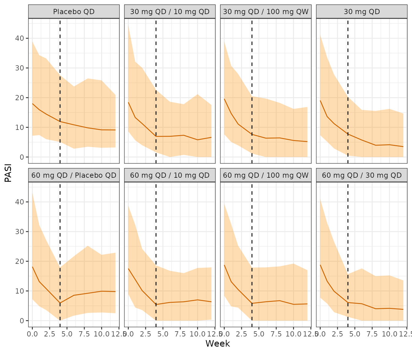
Replicates the simulated percentiles of Figure 3 of Tsamandouras 2024: median and 5th-95th percentiles of PASI by arm. The dashed line marks the end of the induction period.
responders(sim12) |>
  pivot_longer(c(PASI50, PASI75, PASI90, PASI100), names_to = "metric") |>
  mutate(
    regimen = factor(regimen, levels = arm_levels),
    metric = factor(metric, levels = c("PASI50", "PASI75", "PASI90", "PASI100"))
  ) |>
  ggplot(aes(time / 7, value, colour = metric)) +
  geom_line() +
  geom_vline(xintercept = 4, linetype = "dashed") +
  facet_wrap(~regimen, ncol = 4) +
  labs(x = "Week", y = "Responders (%)", colour = NULL) +
  theme_bw() +
  theme(legend.position = "bottom")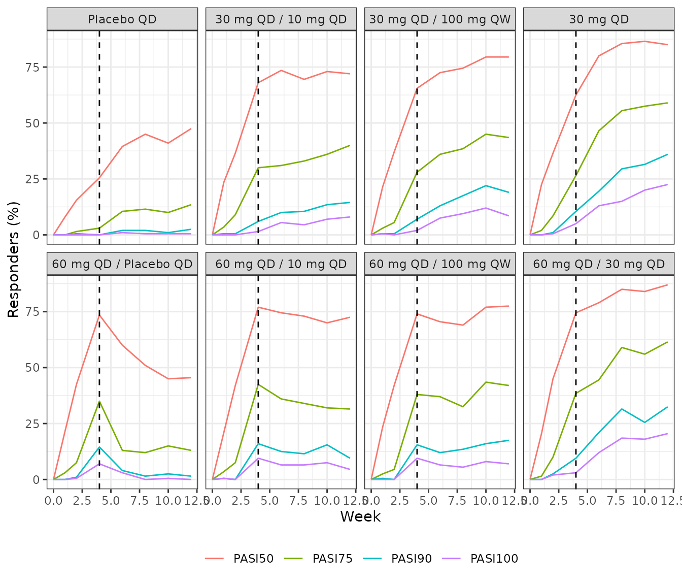
Replicates the model predictions of Figure 4 of Tsamandouras 2024: PASI50/75/90/100 responder rates by arm over the 12-week treatment period.
NCA
The model has no drug concentrations: exposure enters as the
per-period average steady-state concentration CAV, so there
is no concentration-time profile for PKNCA. Validation is against the
paper’s simulated responder rates and median CAV
instead.
Assumptions and deviations
-
Exposure input.
CAVis a covariate in ng/mL, one value per treatment period, computed as Dose / (CL/F x tau) (Eq. 1). The model does not contain the brepocitinib PK model; usemodellib("Hughes_2022_brepocitinib")to derive CL/F, as above. The simulations here use the weight-adjusted typical CL/F with its 78% CV and ignore the other Hughes 2022 covariates (Asian race, food, dose of 175 mg or more), as the paper’s simulations did. - Weights. The paper resampled weights from the study dataset, which is not available; a log-normal distribution with the reported median, truncated to the reported range, stands in for it.
- Fixed-to-zero random effects. The control stream carries etas on Imax, IC50, kout, Pmax and kp with variance fixed at 0; they are omitted, so the only random effect is on the baseline.
-
Imax. Kept as
imax <- fixed(1)because the control stream carries it as a fixed THETA; it does not change any prediction. -
Likelihood.
ll(pasi)reads the observed score fromDVon the 0-72 scale and divides by 72, so the objective function equals the paper’s -2LL. It uses the Nemes approximation to the log gamma function with the control stream’s 3.1415 for pi; the constant cancels from the likelihood’s dependence on the parameters.rxSolve()does not draw from this likelihood, so the vignette draws PASI from the zero-inflated beta distribution in R using thep0_pasi,alpha_pasiandbeta_pasioutputs. - Time. Time is in days from the first dose (kout and kp are per day). The PD switches from the induction to the maintenance exposure at day 28.
-
Placebo. Placebo periods carry
CAV = 0; the placebo effect acts in every arm. - Simulation size. One trial of 200 participants per arm instead of 2000 trials of 56, so the comparisons with Figure 5 carry binomial noise of a few percentage points.