Nusinersen and pNfH neurofilament trafficking in SMA (Paris 2023)
Source:vignettes/articles/Paris_2023_nusinersen_qsp.Rmd
Paris_2023_nusinersen_qsp.RmdModel and source
- Citation: Paris A, Bora P, Parolo S, MacCannell D, Monine M, van der Munnik N, Tong X, Eraly S, Berger Z, Graham D, Ferguson T, Domenici E, Nestorov I, Marchetti L. A pediatric quantitative systems pharmacology model of neurofilament trafficking in spinal muscular atrophy treated with the antisense oligonucleotide nusinersen. CPT Pharmacometrics Syst Pharmacol. 2023;12(2):196-206. doi:10.1002/psp4.12890
- Description: QSP. Paediatric neurofilament-trafficking model of phosphorylated neurofilament heavy subunit (pNfH) in spinal muscular atrophy (SMA), with and without intrathecal nusinersen, from birth to 20 years (Paris 2023). Seven pNfH concentration states (CNS neurons, PNS motor neurons, brain ISF, endoneurial fluid, cranial CSF, spinal CSF, blood) carry first-order synthesis/degradation, leakage and CSF/blood transport, with volume-growth dilution terms from seven growing compartment volumes driven by time-varying body weight (WT) and height (HT). CNS synthesis and leakage follow a synaptic-pruning function of age; SMA adds an age-dependent PNS leakage r14 = A + B * C^(-age). Nusinersen amounts in the three spinal-cord segments come from the embedded nine-compartment Biliouris 2018 PK model (typical rate constants) and pass through a four-stage first-order delay chain whose output inhibits r14 as 1 - ASOeff / (ASOeff + EC50). Model time is postnatal age in days; simulate with covsInterpolation = ‘linear’.
- Article: https://doi.org/10.1002/psp4.12890 (open access, CPT Pharmacometrics Syst Pharmacol 2023;12:196-206)
- Supplement: Appendix S1 (equations, Tables S1-S6) and Appendix S2 (the authors’ complete R source code), both available from the article page.
The model describes phosphorylated neurofilament heavy subunit
(pNfH), a biomarker of axonal damage, from birth to 20 years of age in
children with spinal muscular atrophy (SMA). It extends the authors’
earlier adult neurofilament-trafficking model (Paris 2022) with growing
compartment volumes, a synaptic-pruning description of CNS development,
an extra SMA-driven leak of pNfH from the peripheral nervous system
(reaction r14), and an inhibition of that leak by
intrathecal nusinersen. The nusinersen amount that drives the inhibition
is computed by the nine-compartment Biliouris 2018 PK model (see the
separate Biliouris_2018_nusinersen model), which is
embedded here with its typical rate constants.
Model time is postnatal age in days: every
simulation starts at birth, where the pNfH initial conditions (Table S6)
are defined, and nusinersen doses are placed at the age (in days) at
which they were given. Body weight and height enter as time-varying
covariates and must be solved with
covsInterpolation = "linear", because the volume growth
rates are read off their movement.
Population
The model was parameterised on pNfH measured in CSF and plasma in the Biogen SHINE, NURTURE, EMBRACE, ENDEAR and CHERISH trials (Table S1). 98 healthy paediatric subjects from ENDEAR re-estimated the healthy leakage and blood clearance; 359 SMA patients (17 untreated controls plus the pre-treatment samples of treated patients) defined a 400-member untreated virtual population; 278 treated patients were fitted individually to estimate the treatment parameters; and 25 patients were held out for validation in four age and dose groups (Table S2). Ages ranged from birth to 22 years and intrathecal doses from 1 to 12.5 mg. All fits were normalised least-squares fits of deterministic trajectories, not nonlinear mixed-effects estimation.
ui <- rxode2::rxode(readModelDb("Paris_2023_nusinersen_qsp"))
#> ℹ parameter labels from comments will be replaced by 'label()'
str(ui$population)
#> List of 9
#>  $ species              : chr "human"
#>  $ n_subjects           : num 457
#>  $ n_studies            : num 5
#>  $ age_range            : chr "birth to 22 years (model simulated from birth to 20 years)"
#>  $ disease_state        : chr "Spinal muscular atrophy (SMA), untreated and treated with intrathecal nusinersen; plus healthy paediatric controls"
#>  $ dose_range           : chr "Intrathecal nusinersen 1 to 12.5 mg, individual loading and maintenance schedules"
#>  $ administration_routes: chr "Intrathecal bolus (lumbar puncture) into CSF"
#>  $ regions              : chr "Multinational (Biogen SHINE, NURTURE, EMBRACE, ENDEAR, CHERISH trials)"
#>  $ notes                : chr "98 healthy paediatric subjects (ENDEAR) re-estimated the healthy leakage and blood-clearance rates; 359 SMA pat"| __truncated__
Source trace
Every ini() value carries an in-file comment pointing to
its source in
inst/modeldb/specificDrugs/Paris_2023_nusinersen_qsp.R. The
table collects them. “Code” means the authors’ Appendix S2 R scripts
(pNfH_SMA_model.R,
pNfH_SMA_model_parameters.R,
pNfH_SMA_initial_values.R,
PK_ASO_model.R).
| Equation / parameter | Value | Source location |
|---|---|---|
| pNfH ODEs (7 states) | Eq. S9-S15 | Appendix S1; code NF_SMA_model()
|
| Volume formulas | Formulas S1-S7 | Appendix S1; code (dV_*dt finite-difference block) |
| Pruning function and its use in r1, r3, r5 | Formulas S16-S18 | Appendix S1; code pruning_function(),
pruning_function_der()
|
| r14 = A + B C^(-age) | Equation 1 | Main text; code r14 <- ...
|
| Delay chain and inhibition of r14 | Eq. S20-S24 | Appendix S1; code transit block |
thalf_nf_stat, thalf_nf_mov,
f_nf_stat
|
90 d, 22 d, 0.9 (r2 = r4 = 0.0101/day) | Code; Table S4 r2, r4 |
lk_leak (r5 = r6 base) |
1.7e-6 /day | Table S4, Table S5 |
q_isf_csf, q_endo_csf (r7, r8) |
449.28 mL/day | Table S4 r8; code |
q_cran_spin, q_spin_cran (r9, r10) |
7.4712, 20.148 mL/day | Table S4 |
q_cran_blood, q_spin_blood (r11, r12) |
90, 259.2 mL/day | Table S4 |
lkel_pnfh (r13) |
0.0986 /day | Code (SMA untreated); Table 1 0.10 +/- 0.01 |
r14_a, r14_b, lr14_c
|
1.6e-7 /day, 1.8e-5 /day, 3.3 | Table 1 / Table S4 (untreated population) |
p1_prune … p5_prune
|
-541.49, 0.15976, 527.17, 0.13413, 42.224 | Code; Table S4 |
lktr (kdiff) |
0.09 /day | Table 1 / Table S4 |
lec50 (EC50) |
550 ng | Table 1 / Table S4 |
bl_pnfh_* |
1e5, 2e6, 0.018, 3.4, 1.15, 5.4, 47 ng/mL | Table S6 (SMA untreated column); code |
v0_* |
338, 38.23, 50.7, 25.88, 60, 60, 267.329 mL | Table S3 (birth column); code |
| Nusinersen PK rate constants (16) | K13 … K91, 1/h | Code PK_ASO_model.R (Biliouris 2018 typical
values) |
| Between-subject spread (6 etas) | variances 0.00995 … 0.582 | Table 1 mean +/- SD, moment-matched (see Assumptions) |
Growth inputs
The authors drive volume growth with the CDC clinical growth chart
50th-percentile male weight-for-age and length/stature-for-age curves,
linearly interpolated (Appendix S2, Growth_charts/). The
same 242 knots are reproduced here (birth to 240 months).
# CDC 50th-percentile male weight (kg) and length/stature (cm)
wt <- c(
  3.5302, 4.0031, 4.8795, 5.6729, 6.3914, 7.0418, 7.6304, 8.1630, 8.6448,
  9.0811, 9.4765, 9.8353, 10.1615, 10.4588, 10.7306, 10.9799, 11.2096, 11.4221,
  11.6198, 11.8048, 11.9790, 12.1440, 12.3015, 12.4528, 12.6708, 12.7415, 12.8810,
  13.0184, 13.1545, 13.2899, 13.4252, 13.5609, 13.6974, 13.8351, 13.9742, 14.1150,
  14.2578, 14.4026, 14.5496, 14.6989, 14.8505, 15.0045, 15.1608, 15.3194, 15.4803,
  15.6434, 15.8087, 15.9761, 16.1455, 16.3168, 16.4899, 16.6647, 16.8411, 17.0190,
  17.1984, 17.3791, 17.5610, 17.7440, 17.9281, 18.1132, 18.2991, 18.4859, 18.6735,
  18.8618, 19.0508, 19.2404, 19.4306, 19.6214, 19.8127, 20.0046, 20.1970, 20.3900,
  20.5836, 20.7777, 20.9724, 21.1678, 21.3638, 21.5606, 21.7581, 21.9565, 22.1557,
  22.3558, 22.5570, 22.7593, 22.9627, 23.1674, 23.3734, 23.5809, 23.7898, 24.0003,
  24.2125, 24.4265, 24.6423, 24.8601, 25.0799, 25.3019, 25.5261, 25.7526, 25.9815,
  26.2128, 26.4468, 26.6834, 26.9227, 27.1649, 27.4099, 27.6580, 27.9090, 28.1632,
  28.4206, 28.6813, 28.9453, 29.2127, 29.4836, 29.7580, 30.0360, 30.3177, 30.6031,
  30.8923, 31.1853, 31.4823, 31.7831, 32.0880, 32.3969, 32.7099, 33.0270, 33.3484,
  33.6739, 34.0036, 34.3377, 34.6760, 35.0186, 35.3656, 35.7169, 36.0726, 36.4327,
  36.7970, 37.1658, 37.5388, 37.9162, 38.2978, 38.6836, 39.0736, 39.4678, 39.8660,
  40.2683, 40.6744, 41.0844, 41.4982, 41.9156, 42.3364, 42.7607, 43.1883, 43.6190,
  44.0526, 44.4890, 44.9281, 45.3696, 45.8134, 46.2592, 46.7068, 47.1561, 47.6067,
  48.0585, 48.5111, 48.9644, 49.4181, 49.8719, 50.3255, 50.7786, 51.2310, 51.6823,
  52.1323, 52.5806, 53.0270, 53.4711, 53.9126, 54.3513, 54.7868, 55.2188, 55.6470,
  56.0712, 56.4910, 56.9061, 57.3163, 57.7214, 58.1210, 58.5149, 58.9029, 59.2848,
  59.6603, 60.0293, 60.3916, 60.7470, 61.0954, 61.4366, 61.7706, 62.0972, 62.4164,
  62.7281, 63.0323, 63.3289, 63.6180, 63.8996, 64.1737, 64.4403, 64.6996, 64.9517,
  65.1965, 65.4344, 65.6654, 65.8897, 66.1075, 66.3190, 66.5244, 66.7239, 66.9178,
  67.1064, 67.2899, 67.4686, 67.6428, 67.8128, 67.9788, 68.1411, 68.3000, 68.4558,
  68.6087, 68.7589, 68.9065, 69.0518, 69.1947, 69.3353, 69.4735, 69.6093, 69.7423,
  69.8722, 69.9987, 70.1210, 70.2386, 70.3504, 70.4555, 70.5525, 70.5976
)
ht <- c(
  49.9889, 52.6960, 56.6284, 59.6090, 62.0770, 64.2169, 66.1253, 67.8602, 69.4591,
  70.9480, 72.3459, 73.6667, 74.9213, 76.1184, 77.2648, 78.3662, 79.4273, 80.4521,
  81.4438, 82.4054, 83.3394, 84.2478, 85.1327, 85.9956, 86.4522, 86.8616, 87.6525,
  88.4233, 89.1755, 89.9104, 90.6291, 91.3324, 92.0213, 92.6964, 93.3585, 94.0082,
  94.6464, 95.2736, 95.9147, 96.5473, 97.1719, 97.7890, 98.3990, 99.0025, 99.6000,
  100.1918, 100.7783, 101.3600, 101.9373, 102.5105, 103.0799, 103.6459, 104.2087, 104.7687,
  105.3262, 105.8813, 106.4343, 106.9855, 107.5350, 108.0830, 108.6296, 109.1751, 109.7196,
  110.2631, 110.8058, 111.3477, 111.8890, 112.4296, 112.9696, 113.5090, 114.0479, 114.5861,
  115.1238, 115.6609, 116.1973, 116.7329, 117.2678, 117.8018, 118.3348, 118.8668, 119.3977,
  119.9272, 120.4554, 120.9821, 121.5072, 122.0305, 122.5520, 123.0714, 123.5886, 124.1035,
  124.6160, 125.1259, 125.6331, 126.1374, 126.6388, 127.1370, 127.6320, 128.1237, 128.6119,
  129.0966, 129.5777, 130.0550, 130.5286, 130.9983, 131.4641, 131.9260, 132.3840, 132.8381,
  133.2882, 133.7345, 134.1769, 134.6155, 135.0504, 135.4818, 135.9097, 136.3343, 136.7557,
  137.1742, 137.5899, 138.0032, 138.4143, 138.8234, 139.2310, 139.6373, 140.0427, 140.4477,
  140.8527, 141.2582, 141.6646, 142.0725, 142.4824, 142.8949, 143.3107, 143.7304, 144.1545,
  144.5838, 145.0190, 145.4607, 145.9097, 146.3665, 146.8320, 147.3066, 147.7911, 148.2859,
  148.7917, 149.3088, 149.8376, 150.3784, 150.9313, 151.4964, 152.0735, 152.6624, 153.2627,
  153.8738, 154.4951, 155.1255, 155.7642, 156.4099, 157.0612, 157.7168, 158.3751, 159.0344,
  159.6931, 160.3493, 161.0015, 161.6478, 162.2865, 162.9161, 163.5350, 164.1418, 164.7352,
  165.3140, 165.8771, 166.4236, 166.9528, 167.4641, 167.9571, 168.4313, 168.8867, 169.3231,
  169.7405, 170.1393, 170.5195, 170.8815, 171.2257, 171.5525, 171.8626, 172.1563, 172.4343,
  172.6972, 172.9456, 173.1801, 173.4014, 173.6101, 173.8067, 173.9920, 174.1665, 174.3308,
  174.4854, 174.6310, 174.7680, 174.8969, 175.0182, 175.1323, 175.2398, 175.3410, 175.4362,
  175.5259, 175.6104, 175.6901, 175.7652, 175.8360, 175.9028, 175.9658, 176.0254, 176.0816,
  176.1348, 176.1850, 176.2326, 176.2776, 176.3202, 176.3606, 176.3989, 176.4352, 176.4697,
  176.5024, 176.5335, 176.5630, 176.5911, 176.6179, 176.6433, 176.6676, 176.6907, 176.7127,
  176.7337, 176.7538, 176.7730, 176.7913, 176.8088, 176.8255, 176.8415, 176.8492
)
cdc <- data.frame(
  age_mo = c(0, seq(0.5, 22.5, 1), 24, seq(24.5, 239.5, 1), 240),
  wt = wt,
  ht = ht
)
stopifnot(nrow(cdc) == length(wt), nrow(cdc) == length(ht))

cdc_wt <- function(age_yr) approx(cdc$age_mo / 12, cdc$wt, age_yr, rule = 2)$y
cdc_ht <- function(age_yr) approx(cdc$age_mo / 12, cdc$ht, age_yr, rule = 2)$y

# One subject from birth: observation rows on `grid` (days), nusinersen
# doses (mg) at `dose_day`, and CDC-median covariates on every row. `lead`
# shifts the covariate lookup forward in age (in years).
make_events <- function(grid, dose_day = numeric(0), dose_mg = numeric(0),
                        id = 1L, lead = 0) {
  obs <- data.frame(time = grid, evid = 0L, amt = 0, cmt = "pnfh_blood")
  dos <- data.frame(time = dose_day, evid = rep(1L, length(dose_day)),
                    amt = dose_mg, cmt = rep("csf", length(dose_day)))
  bind_rows(obs, dos) |>
    mutate(id = id,
           WT = cdc_wt(time / 365 + lead),
           HT = cdc_ht(time / 365 + lead)) |>
    arrange(time, desc(evid)) |>
    select(id, time, evid, amt, cmt, WT, HT)
}

# The model has no residual-error block, so rxSolve() warns "No sigma
# parameters", and a zeroRe() model notes that its etas are zero; muffle
# only those two conditions.
solve_model <- function(model, events, ...) {
  withCallingHandlers(
    rxode2::rxSolve(model, events, covsInterpolation = "linear",
                    returnType = "data.frame", ...),
    warning = function(w) {
      if (grepl("No sigma", conditionMessage(w))) invokeRestart("muffleWarning")
    },
    message = function(m) {
      if (grepl("treated as zero", conditionMessage(m))) invokeRestart("muffleMessage")
    }
  )
}

mod_typ <- rxode2::zeroRe(ui)
#> Warning: No sigma parameters in the model

# Healthy paediatric scenario: no SMA leak, healthy blood clearance and
# healthy birth concentrations (Table S6 healthy column, code
# 'healthy_pediatric').
healthy <- c(r14_a = 0, r14_b = 0, lkel_pnfh = log(0.33),
             bl_pnfh_endo = 0.05, bl_pnfh_csf_cranial = 0.1,
             bl_pnfh_csf_spinal = 0.18, bl_pnfh_blood = 0.8)
Agreement with the authors’ deposited code
The authors’ R code was run with deSolve (lsodes) for its three
built-in scenarios: healthy, average SMA untreated, and its example
treatment (12 mg at ages 1 year + 0, 14, 77, 250, 375, 500, 625, 750,
875 and 1000 days, with EC50 = 550, the Table 1 estimate).
The pNfH concentrations it produced at selected ages are tabulated below
and compared with this model. The code evaluates body weight and height
one day ahead of the current age (its finite-difference step), so the
comparison feeds the covariates with the same one-day lead, and uses the
code’s healthy blood value at birth (8 ng/mL; see Assumptions).
ref_untx <- data.frame(
  day = c(91, 182, 365, 730, 1095, 1825, 3650, 5475, 7300),
  h_csf = c(99.5, 123.0, 173.7, 265.1, 340.2, 458.5, 613.5, 675.0, 622.4),
  h_blood = c(250.7, 257.7, 286.6, 331.3, 370.3, 384.5, 285.6, 175.3, 141.8),
  u_csf = c(4342.7, 3994.1, 3197.2, 1754.9, 1037.8, 751.8, 920.2, 1014.5, 936.4),
  u_blood = c(26081.9, 18428.7, 11267.7, 4960.5, 2809.7, 1791.3, 1260.0, 784.8, 637.5)
)
ref_tx <- data.frame(
  day = 365 + c(14, 30, 60, 100, 365, 1000),
  csf = c(240.5, 188.4, 191.4, 201.4, 265.9, 389.1),
  blood = c(5513.6, 1930.9, 1034.4, 1004.0, 1104.4, 1281.0)
)

ev_id <- make_events(0:7300, lead = 1 / 365)
sim_h <- solve_model(mod_typ, ev_id, params = c(healthy, bl_pnfh_blood = 8))
sim_u <- solve_model(mod_typ, ev_id)

dose_day_ex <- 365 + c(0, 14, 77, 250, 375, 500, 625, 750, 875, 1000)
ev_tx <- make_events(0:1825, dose_day_ex, rep(12, 10), lead = 1 / 365)
sim_tx <- solve_model(mod_typ, ev_tx)

at <- function(sim, day, col) sim[[col]][match(day, sim$time)]
cmp_untx <- ref_untx |>
  mutate(
    h_csf_sim = at(sim_h, day, "pnfh_csf_pgml"),
    h_blood_sim = at(sim_h, day, "pnfh_blood_pgml"),
    u_csf_sim = at(sim_u, day, "pnfh_csf_pgml"),
    u_blood_sim = at(sim_u, day, "pnfh_blood_pgml")
  )
cmp_tx <- ref_tx |>
  mutate(csf_sim = at(sim_tx, day, "pnfh_csf_pgml"),
         blood_sim = at(sim_tx, day, "pnfh_blood_pgml"))

cmp_untx |>
  mutate(age_years = round(day / 365, 2)) |>
  select(age_years, h_csf, h_csf_sim, h_blood, h_blood_sim,
         u_csf, u_csf_sim, u_blood, u_blood_sim) |>
  mutate(across(-age_years, \(x) signif(x, 4))) |>
  rename("Age (years)" = age_years,
         "Healthy CSF, code" = h_csf, "Healthy CSF, model" = h_csf_sim,
         "Healthy blood, code" = h_blood, "Healthy blood, model" = h_blood_sim,
         "SMA CSF, code" = u_csf, "SMA CSF, model" = u_csf_sim,
         "SMA blood, code" = u_blood, "SMA blood, model" = u_blood_sim) |>
knitr::kable(caption = "pNfH (pg/mL) in spinal CSF and blood, healthy and SMA untreated.")| Age (years) | Healthy CSF, code | Healthy CSF, model | Healthy blood, code | Healthy blood, model | SMA CSF, code | SMA CSF, model | SMA blood, code | SMA blood, model |
|---|---|---|---|---|---|---|---|---|
| 0.25 | 99.5 | 99.45 | 250.7 | 250.7 | 4343.0 | 4343.0 | 26080.0 | 26080.0 |
| 0.50 | 123.0 | 123.00 | 257.7 | 257.7 | 3994.0 | 3994.0 | 18430.0 | 18430.0 |
| 1.00 | 173.7 | 173.70 | 286.6 | 286.6 | 3197.0 | 3197.0 | 11270.0 | 11270.0 |
| 2.00 | 265.1 | 265.10 | 331.3 | 331.3 | 1755.0 | 1755.0 | 4960.0 | 4960.0 |
| 3.00 | 340.2 | 340.20 | 370.3 | 370.3 | 1038.0 | 1038.0 | 2810.0 | 2810.0 |
| 5.00 | 458.5 | 458.50 | 384.5 | 384.5 | 751.8 | 751.8 | 1791.0 | 1791.0 |
| 10.00 | 613.5 | 613.60 | 285.6 | 285.6 | 920.2 | 920.2 | 1260.0 | 1260.0 |
| 15.00 | 675.0 | 675.00 | 175.3 | 175.3 | 1014.0 | 1014.0 | 784.8 | 784.8 |
| 20.00 | 622.4 | 623.20 | 141.8 | 141.9 | 936.4 | 937.1 | 637.5 | 637.9 |
cmp_tx |>
  mutate(days_after_first_dose = day - 365) |>
  select(days_after_first_dose, csf, csf_sim, blood, blood_sim) |>
  mutate(across(c(csf_sim, blood_sim), \(x) signif(x, 4))) |>
  rename("Days after first dose" = days_after_first_dose,
         "CSF, code" = csf, "CSF, model" = csf_sim,
         "Blood, code" = blood, "Blood, model" = blood_sim) |>
knitr::kable(caption = "pNfH (pg/mL) during the authors' example treatment from age 1 year.")| Days after first dose | CSF, code | CSF, model | Blood, code | Blood, model |
|---|---|---|---|---|
| 14 | 240.5 | 240.5 | 5513.6 | 5513 |
| 30 | 188.4 | 188.4 | 1930.9 | 1931 |
| 60 | 191.4 | 191.4 | 1034.4 | 1034 |
| 100 | 201.4 | 201.4 | 1004.0 | 1004 |
| 365 | 265.9 | 265.9 | 1104.4 | 1104 |
| 1000 | 389.1 | 389.1 | 1281.0 | 1281 |
rel_err <- c(
  with(cmp_untx, abs(c(h_csf_sim / h_csf, h_blood_sim / h_blood,
                       u_csf_sim / u_csf, u_blood_sim / u_blood) - 1)),
  with(cmp_tx, abs(c(csf_sim / csf, blood_sim / blood) - 1))
)
# Same equations and parameters on both sides; the residual difference is
# integrator tolerance plus the rounding of the tabulated reference to one
# decimal place.
stopifnot(!anyNA(rel_err), max(rel_err) < 0.005)
The embedded nusinersen PK can be checked the same way: the authors’
PK_ASO_model() returns 549,299, 706,509, 761,354 and
743,796 ng of nusinersen summed over the three spinal-cord segments 0.5,
1, 2 and 7 days after a single 12 mg dose.
sim_pk <- solve_model(mod_typ, make_events(c(0, 0.5, 1, 2, 7), 0, 12))
aso_ref <- c(549299.1, 706508.5, 761353.6, 743795.9)
aso_sim <- at(sim_pk, c(0.5, 1, 2, 7), "aso_sc")
data.frame(day = c(0.5, 1, 2, 7), code = aso_ref, model = signif(aso_sim, 7)) |>
  rename("Days after dose" = day, "Spinal-cord nusinersen, code (ng)" = code,
         "Spinal-cord nusinersen, model (ng)" = model) |>
knitr::kable()| Days after dose | Spinal-cord nusinersen, code (ng) | Spinal-cord nusinersen, model (ng) |
|---|---|---|
| 0.5 | 549299.1 | 549299.1 |
| 1.0 | 706508.5 | 706508.5 |
| 2.0 | 761353.6 | 761353.6 |
| 7.0 | 743795.9 | 743795.9 |
Volume growth (Figure S1, Table S3)
grid <- seq(0, 7300, 7)
sim_u_w <- solve_model(mod_typ, make_events(grid))
sim_h_w <- solve_model(mod_typ, make_events(grid), params = healthy)

vol_long <- sim_u_w |>
  select(time, starts_with("vol_")) |>
  pivot_longer(-time, names_to = "compartment", values_to = "volume")
ggplot(vol_long, aes(time / 365, volume)) +
  geom_line() +
  facet_wrap(~compartment, scales = "free_y") +
  labs(x = "Age (years)", y = "Volume (mL)",
       caption = "Replicates Figure S1 of Paris 2023.")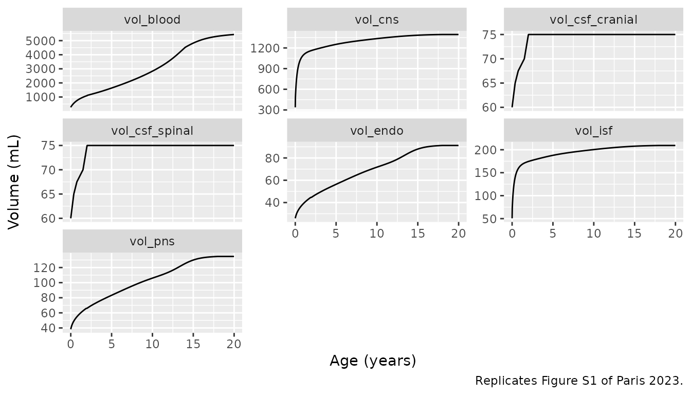
vol20 <- sim_u_w |> filter(time == max(time)) |> select(starts_with("vol_"))
tab_s3 <- data.frame(
  compartment = c("vol_cns", "vol_pns", "vol_isf", "vol_endo",
                  "vol_csf_cranial", "vol_csf_spinal", "vol_blood"),
  table_s3 = c(1413, 135, 209, 91, 75, 75, 5436)
) |>
  mutate(model = signif(unlist(vol20[compartment]), 5),
         pct_diff = round(100 * (model / table_s3 - 1), 1))
tab_s3 |>
  rename("Compartment" = compartment, "Table S3, 20 years (mL)" = table_s3,
         "Model, 20 years (mL)" = model, "Difference (%)" = pct_diff) |>
knitr::kable()| Compartment | Table S3, 20 years (mL) | Model, 20 years (mL) | Difference (%) |
|---|---|---|---|
| vol_cns | 1413 | 1395.100 | -1.3 |
| vol_pns | 135 | 134.710 | -0.2 |
| vol_isf | 209 | 209.270 | 0.1 |
| vol_endo | 91 | 91.189 | 0.2 |
| vol_csf_cranial | 75 | 75.000 | 0.0 |
| vol_csf_spinal | 75 | 75.000 | 0.0 |
| vol_blood | 5436 | 5435.300 | 0.0 |
Healthy and untreated SMA trajectories (Figure 2)
fig2 <- bind_rows(
  sim_h_w |> mutate(scenario = "Healthy"),
  sim_u_w |> mutate(scenario = "SMA untreated (average)")
) |>
  select(time, scenario, "CSF spinal pNfH" = pnfh_csf_pgml,
         "Blood pNfH" = pnfh_blood_pgml) |>
  pivot_longer(c("CSF spinal pNfH", "Blood pNfH"),
               names_to = "matrix", values_to = "pnfh")
ggplot(fig2, aes(time / 365, pnfh, colour = scenario)) +
  geom_line() +
  scale_y_log10() +
  facet_wrap(~matrix, scales = "free_y") +
  labs(x = "Age (years)", y = "pNfH (pg/mL)", colour = NULL,
       caption = "Replicates the typical curves of Figure 2 of Paris 2023.") +
  theme(legend.position = "bottom")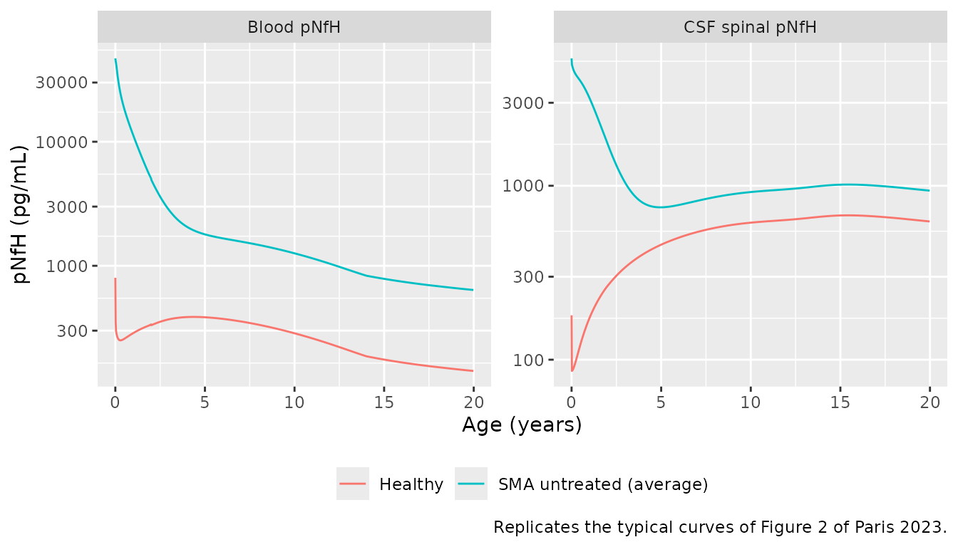
As in Figure 2, the average SMA trajectory starts far above the
healthy one (47,000 vs about 800 pg/mL in blood at birth, Table S6),
falls steeply over the first two years as the age-dependent part of
r14 decays, and settles within a few-fold of the healthy
curve in later childhood.
r14 <- sim_u_w |>
  transmute(age = time / 365, Total = r14, `Age-independent term (A)` = r14a,
            `Age-dependent term (B C^-age)` = r14 - r14a) |>
  pivot_longer(-age, names_to = "term", values_to = "rate")
ggplot(r14, aes(age, rate, linetype = term)) +
  geom_line() +
  scale_y_log10() +
  labs(x = "Age (years)", y = "r14 (1/day)", linetype = NULL,
       caption = "Replicates Figure S2 of Paris 2023.") +
  theme(legend.position = "bottom")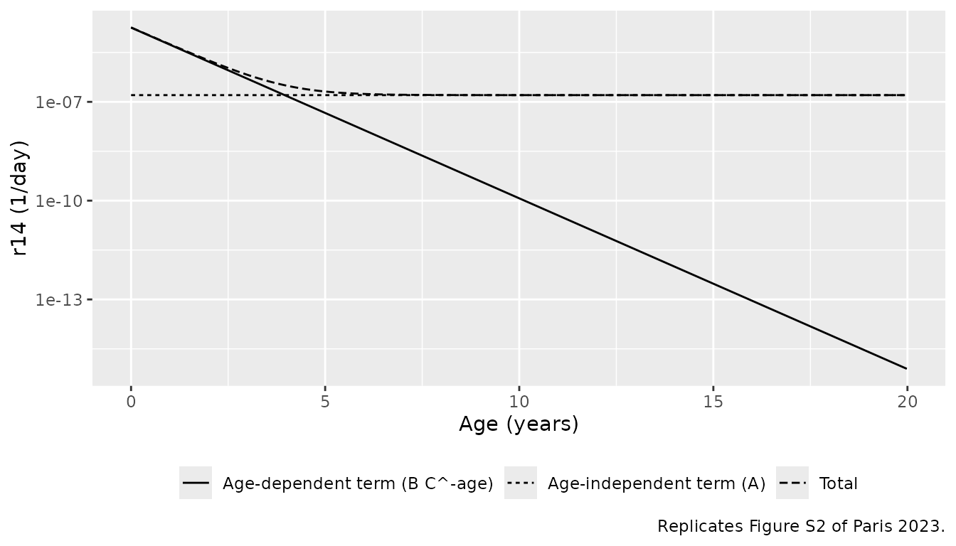
Treatment: delay and potency
The four-stage delay chain has a mean transit time of
4 / kdiff:
kdiff <- exp(ui$theta[["lktr"]])
c(kdiff_per_day = kdiff, mean_transit_days = 4 / kdiff)
#>     kdiff_per_day mean_transit_days
#>           0.09000          44.44444
stopifnot(abs(4 / kdiff - 44.4) < 0.1)
The paper describes this as “an average time delay of approximately 40 days” between the input and the effective drug signal.
EC50 is printed as 5.5 x 10^2 in both Table 1 and Table S4, while the authors’ example script uses 5.5 x 10^3. Because the spinal-cord nusinersen amount after a 12 mg dose (about 7 x 10^5 ng) is three orders of magnitude above either value, the choice matters only in the first two to three weeks after the first dose:
sim_tx_hi <- solve_model(mod_typ, make_events(0:1825, dose_day_ex, rep(12, 10)),
                         params = c(lec50 = log(5500)))
sim_tx_lo <- solve_model(mod_typ, make_events(0:1825, dose_day_ex, rep(12, 10)))
ec50_cmp <- bind_rows(
  sim_u |> filter(time <= 1825) |> mutate(scenario = "Untreated"),
  sim_tx_lo |> mutate(scenario = "Treated, EC50 = 550"),
  sim_tx_hi |> mutate(scenario = "Treated, EC50 = 5500")
)
ggplot(filter(ec50_cmp, time >= 300), aes(time / 365, pnfh_blood_pgml, colour = scenario)) +
  geom_line() +
  scale_y_log10() +
  labs(x = "Age (years)", y = "Blood pNfH (pg/mL)", colour = NULL,
       caption = "12 mg loading and maintenance from age 1 year (the authors' example).") +
  theme(legend.position = "bottom")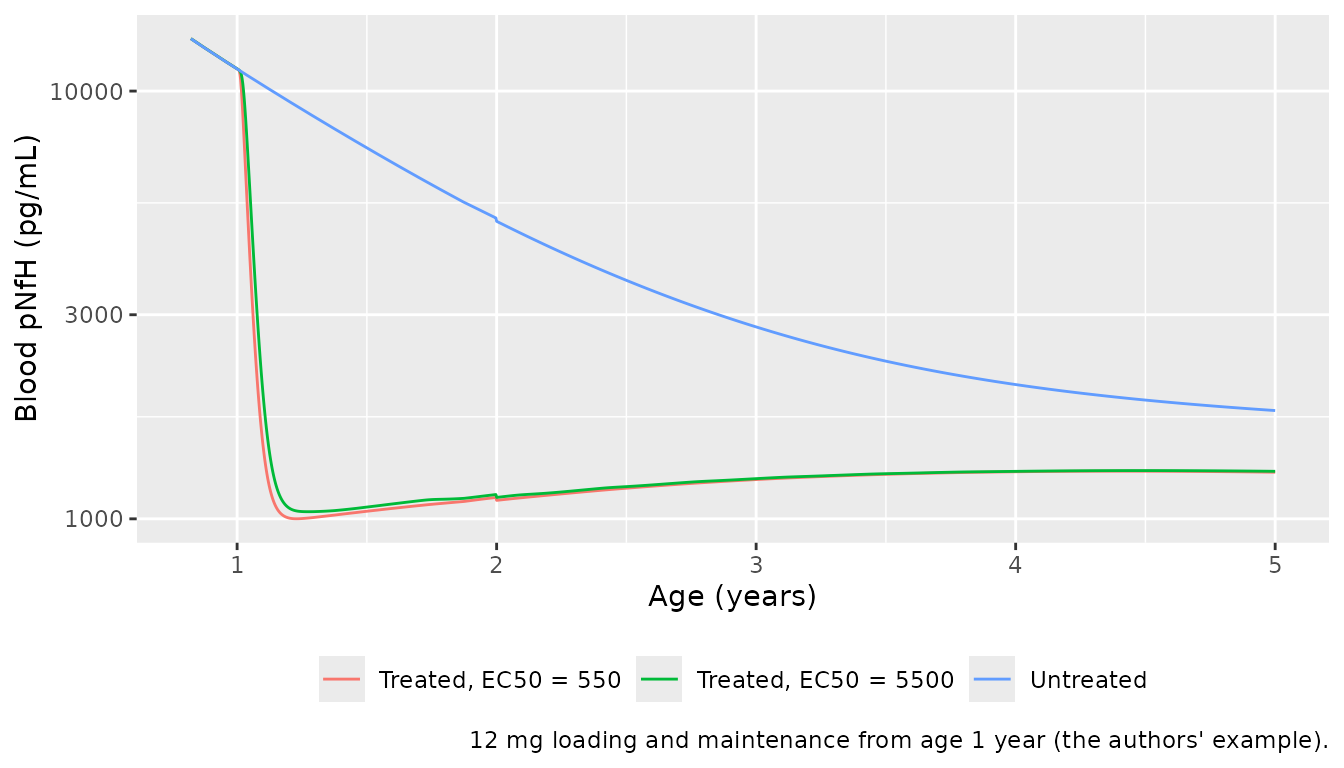
Validation groups (Table S2, Figure 5)
Table S2 gives the median dosing schedule and the mean age at the first dose for the four held-out validation groups. Each is simulated here from birth, untreated and treated, as the typical subject and as a cohort of 100 virtual patients drawing the between-subject spread from Table 1. The paper additionally rescaled its 300 sampled curves so their mean matched each group’s mean measured pNfH before treatment, a step that depends on the measured data and is not reproduced; the bands below are therefore the model’s prior spread for a subject of that age, not the paper’s refined bands.
groups <- list(
  list(name = "Group 1 (age 0.61 y, plasma)", age = 0.61, end = 2.5,
       day = c(0, 14, 28, 63), mg = c(10.8, 10.8, 10.8, 10.8)),
  list(name = "Group 2 (age 0.36 y, plasma)", age = 0.36, end = 2.5,
       day = c(0, 14, 28), mg = c(10.3, 10.3, 11.8)),
  list(name = "Group 3 (age 0.31 y, CSF + plasma)", age = 0.31, end = 5,
       day = c(0, 14, 28, 56, 184, 297, 428, 590, 703, 836, 954),
       mg = c(10.3, 10.3, 10.3, 10.3, 10.8, 11.3, 11.3, 11.3, 12, 12, 12)),
  list(name = "Group 4 (age 1.4 y, CSF + plasma)", age = 1.4, end = 7,
       day = c(0, 14, 28, 64, 182, 302, 1031, 1155, 1268),
       mg = c(11.3, 11.3, 11.3, 11.3, 11.3, 12, 12, 12, 12))
)

n_cohort <- 100
rxode2::rxSetSeed(20230215)
grp_typ <- list()
grp_vpc <- list()
for (g in groups) {
  grid_g <- seq(0, round(g$end * 365), 7)
  dose_g <- round(g$age * 365) + g$day
  ev_untx <- make_events(grid_g)
  ev_tx_g <- make_events(grid_g, dose_g, g$mg)
  grp_typ[[g$name]] <- bind_rows(
    solve_model(mod_typ, ev_untx) |> mutate(arm = "Untreated"),
    solve_model(mod_typ, ev_tx_g) |> mutate(arm = "Treated")
  ) |>
    mutate(group = g$name, start = g$age)
  ev_tx_n <- bind_rows(lapply(seq_len(n_cohort), \(i) make_events(grid_g, dose_g, g$mg, id = i)))
  grp_vpc[[g$name]] <- solve_model(ui, ev_tx_n) |>
    group_by(time) |>
    summarise(lo = quantile(pnfh_blood_pgml, 0.025),
              med = median(pnfh_blood_pgml),
              hi = quantile(pnfh_blood_pgml, 0.975), .groups = "drop") |>
    mutate(group = g$name, start = g$age)
}
grp_typ <- bind_rows(grp_typ)
grp_vpc <- bind_rows(grp_vpc)

ggplot() +
  geom_ribbon(data = filter(grp_vpc, time / 365 > start - 0.3), aes(time / 365, ymin = lo, ymax = hi),
              fill = "steelblue", alpha = 0.25) +
  geom_line(data = filter(grp_typ, time / 365 > start - 0.3),
            aes(time / 365, pnfh_blood_pgml, colour = arm)) +
  facet_wrap(~group, scales = "free") +
  scale_colour_manual(values = c(Treated = "blue", Untreated = "orange")) +
  labs(x = "Age (years)", y = "Blood pNfH (pg/mL)", colour = "Typical subject",
       caption = paste("Shaded: 2.5th-97.5th percentile of 100 treated virtual patients.",
                       "Compare Figure 5 (a, b, d, f) of Paris 2023.")) +
  theme(legend.position = "bottom")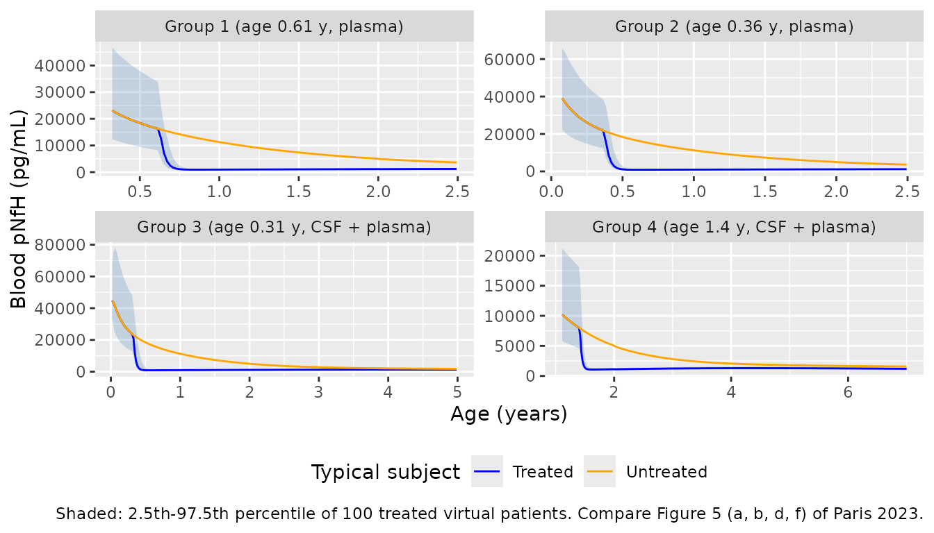
ggplot(filter(grp_typ, grepl("Group [34]", group), time / 365 > start - 0.3),
       aes(time / 365, pnfh_csf_pgml, colour = arm)) +
  geom_line() +
  facet_wrap(~group, scales = "free") +
  scale_colour_manual(values = c(Treated = "blue", Untreated = "orange")) +
  labs(x = "Age (years)", y = "Spinal CSF pNfH (pg/mL)", colour = "Typical subject",
       caption = "Compare Figure 5 (c, e) of Paris 2023.") +
  theme(legend.position = "bottom")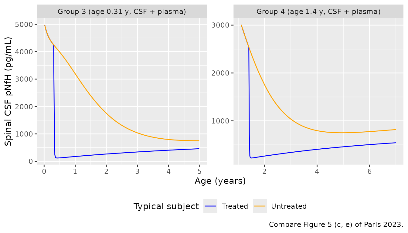
Figure 5 shows blood pNfH falling within roughly two months of the first dose from the 10,000-20,000 pg/mL range to near 1,000 pg/mL, with the untreated mean declining only slowly. The typical treated subject reproduces that drop:
grp_ratio <- grp_typ |>
  mutate(t_after = time - round(start * 365)) |>
  filter(t_after >= 84, t_after < 91) |>
  group_by(group) |>
  summarise(
    blood_untreated = pnfh_blood_pgml[arm == "Untreated"][1],
    blood_treated = pnfh_blood_pgml[arm == "Treated"][1],
    .groups = "drop"
  ) |>
  mutate(ratio = blood_treated / blood_untreated)
grp_ratio |>
  mutate(across(where(is.numeric), \(x) signif(x, 3))) |>
  rename("Group" = group, "Untreated (pg/mL)" = blood_untreated,
         "Treated (pg/mL)" = blood_treated, "Treated / untreated" = ratio) |>
knitr::kable(caption = "Typical blood pNfH about 12 weeks after the first dose.")| Group | Untreated (pg/mL) | Treated (pg/mL) | Treated / untreated |
|---|---|---|---|
| Group 1 (age 0.61 y, plasma) | 13000 | 927 | 0.0714 |
| Group 2 (age 0.36 y, plasma) | 16600 | 878 | 0.0529 |
| Group 3 (age 0.31 y, CSF + plasma) | 17300 | 868 | 0.0502 |
| Group 4 (age 1.4 y, CSF + plasma) | 6640 | 1070 | 0.1610 |
Non-compartmental analysis
There is no NCA comparison: the paper reports no exposure metrics, and the model’s outputs are endogenous biomarker concentrations that start at a non-zero birth value rather than drug concentrations after a dose. The embedded nusinersen PK is validated against the authors’ code above, and the whole system is validated against the trajectories the authors’ code produces.
Assumptions and deviations
-
The deposited code is followed where it disagrees with the
printed tables. Appendix S2 is described by the authors as the
complete source code of the model; it reproduces Figure 2, and its
values are used here. The disagreements are:
- Pruning rates: the code has P2 = 0.1597563 and P4 = 0.1341329; Table S4 prints 0.161 and 0.131. P1, P3 and P5 in Table S4 are exact roundings of the code values, P2 and P4 are not. With the Table S4 values every pNfH concentration (CNS, spinal CSF, blood) is up to about 8% higher.
- r7: Table S4 prints 0.33; the code uses 449.28 mL/day, and Table S4 itself gives r8 = 449.28 mL/day “assumed equal to r7”.
- r1 and r3: Table S4 prints 12300.21 ng/(mL day); the code (and the Table S4 description “at equilibrium with degradation for the initial concentration”) sets them to r2 times the birth concentration, about 1008 ng/(mL day) for the CNS. The code also applies the pruning shape to r3, where Formula S17 names only r1.
- CSF volumes: Formulas S5 and S6 are printed as steps (60, 65, 67.7, 70, 75 mL); the code interpolates linearly through 60, 65, 67.5, 70 and 75 mL at 0, 0.375, 0.75, 1.5 and 2 years. The linear form is used because a step would put an instantaneous dilution in the concentration equations.
- CNS volume at 20 years: Table S3 prints 1413 mL; the code gives 1395 mL (see the Table S3 comparison above).
- Healthy blood pNfH at birth: Table S6 gives 800 pg/mL, the code 8 ng/mL (8000 pg/mL). With a blood half-life of about 2 days the two converge within the first weeks; the Table S6 value is used for the healthy scenario except in the code comparison.
- Volumes at birth do not equal the growth formulas at birth. The birth volumes (Table S3) are the code’s initial conditions; the formulas evaluated at the CDC birth weight give a larger CNS (424 vs 338 mL) and blood (282 vs 267 mL) volume, and the volume states relax onto them within hours. That relaxation dilutes the CNS pNfH by about 23% on the first day of life. This is the authors’ implementation and is kept.
- Volume dynamics. The code relaxes each volume onto its target at 365 per day (its finite-difference step of one day, expressed in years), with the target evaluated one day ahead in age. Here the CSF and blood formula switches use the same one-day lead, but body weight and height are read at the current time, so supply them at the subject’s age. The neural and CSF volumes stop growing at 18 years and the blood volume at 20.
-
EC50 units. Tables 1 and S4 give EC50 in ng/mL, but
the driver of the delay chain is the summed nusinersen amount
(ng) in the three spinal-cord compartments of the PK model (Appendix S1,
Eq. S20; code
PK_ASO_model()), so EC50 is an amount. The Table 1 value 550 is used; the code’s example script uses 5500 (compared above). - Embedded nusinersen PK. The code uses the Biliouris 2018 typical rate constants without the body-weight scaling and between-subject variability of the published PK model, although the main text says the PK model was translated to children allometrically. The code’s version is used. The code’s dosing helper adds the first dose’s amount at every dosing time; this model doses the amount given, which only matters for schedules with unequal doses such as those of Table S2.
-
Default parameter set. The defaults are the code’s
average SMA untreated scenario (r13 and r14 from the untreated virtual
population, Table 1 first column) with the treatment parameters from the
individual treatment fits (Table 1 second column), as in the authors’
example script. The treatment-fit means for r13 and r14 (0.12 /day;
1.04e-7 /day, 1.56e-5 /day, 3.25) can be supplied through
params. -
Between-subject spread. The paper reports parameter
distributions as mean +/- SD of the 400-member untreated virtual
population and of the individual treatment fits (Table 1), not as
estimated random effects. They are encoded as independent log-normal
etas whose variance
log(1 + (SD / mean)^2)matches each CV (r13 10%, r14A 62.5%, r14B 33%, r14C 27%, EC50 38%, kdiff 89%). The shape of the distributions and their correlations are not reported. There is no residual-error model; the paper fitted with normalised least squares and reports no residual variance. -
Growth curves. The CDC 50th-percentile male curves
are the authors’ default for every subject; sex-specific or individual
curves can be supplied as
WTandHT. - Newborns. The paper notes the model underpredicts CSF pNfH in the first three months of life (NURTURE newborns were excluded from the treatment training set).