Ribavirin (Mulder 2025)
Source:vignettes/articles/Mulder_2025_ribavirin.Rmd
Mulder_2025_ribavirin.RmdModel and source
- Citation: Mulder MB, van Noort M, de Man RA, Kamar N, de Bruijne J, Knoester M, Blokzijl H, Vanwolleghem T, Roosens L, Izopet J, Gandia P, van der Eijk AA, Metselaar HJ, Ahsman MJ, van Steeg TJ, Hesselink DA, de Winter BCM. (2025). Development of a ribavirin dosing regimen in transplant recipients with chronic hepatitis E virus infection: a population pharmacokinetic and -dynamic model. J Antimicrob Chemother 80(8):2158-2168. doi:10.1093/jac/dkaf183. PMID 40581807. PK structural parameters Ka, Vc, Q, and Vp and the WT and SEXF effects on Vc and Vp are fixed from Wu LS, Rower JE, Burton JR Jr et al. (2015) Antimicrob Agents Chemother 59:2179-2188 (doi:10.1128/AAC.04618-14; the reference weight 79 kg is taken from Wu 2015 Table 2 / covariate-equation form). Infected and healthy hepatocyte half-lives derive from Dahari H, Lo A, Ribeiro RM et al. (2007) J Theor Biol 247:371-381 (doi:10.1016/j.jtbi.2007.03.006).
- Article: https://doi.org/10.1093/jac/dkaf183
- Upstream PK reference (Wu 2015): https://doi.org/10.1128/AAC.04618-14
- Hepatocyte-kinetics reference (Dahari 2007): https://doi.org/10.1016/j.jtbi.2007.03.006
This is the first nlmixr2lib model file describing the population pharmacokinetics and -dynamics of ribavirin in solid organ transplant (SOT) recipients with chronic hepatitis E virus (HEV) infection. The integrated model couples a two-compartment population PK model (most parameters fixed from a prior HCV ribavirin popPK fit, Wu 2015) to two PD endpoints: an indirect-response model for haemoglobin (toxicity) and a target-cell-limited three-compartment model for HEV viral load (efficacy).
Population
The source paper analysed data from 107 chronically HEV-infected SOT recipients (32.7% female; age median 56.9 years, range 22-84; body weight median 74 kg, range 43.5-140) treated with oral ribavirin at a median dose of 600 mg/day (range 100-2400) for a median 90 days (range 21-1333) between September 2009 and November 2019. Renal function was widely variable (eGFR median 50 mL/min/1.73 m^2, range 6-117), reflecting the heterogeneous SOT population (kidney 43.9%, liver 17.8%, heart 14.9%, lung 14%, multi-organ 8.4%). Most subjects were on tacrolimus-based immunosuppression. Sustained virologic response (SVR) was achieved in 68.2% of subjects (Mulder 2025 Table 1).
The same information is available programmatically via
readModelDb("Mulder_2025_ribavirin")()$population.
Source trace
The per-parameter origin is recorded as an in-file comment next to
each ini() entry in
inst/modeldb/specificDrugs/Mulder_2025_ribavirin.R. The
table below collects them in one place for review.
| Equation / parameter | Value (typical) | Source location |
|---|---|---|
lka (absorption rate ka) |
2.91 h^-1 (fixed) | Mulder 2025 Table 2 “K a (h-1)” – Wu 2015 starting model |
lcl (clearance CL/F) |
26.4 L/h (re-estimated) | Mulder 2025 Table 2 “CL (L/h)” |
lvc (central volume Vc/F = V2) |
769 L (fixed) | Mulder 2025 Table 2 “V2 (L)” – Wu 2015 starting model |
lq (intercompartmental clearance Q/F = Q1) |
104 L/h (fixed) | Mulder 2025 Table 2 “Q1 (L/h)” – Wu 2015 starting model |
lvp (peripheral volume Vp/F = V3) |
3570 L (fixed) | Mulder 2025 Table 2 “V3 (L)” – Wu 2015 starting model |
e_crcl_cl (CRCL effect on CL exponent) |
1.32 | Mulder 2025 Table 2 “eGFR on Cl” |
crcl_ref (CRCL cap / centring threshold) |
57 mL/min/1.73 m^2 | Mulder 2025 Table 2 “Cut-off value on kidney function (mL/min)” |
e_wt_vc (WT exponent on Vc) |
1.29 (fixed) | Mulder 2025 Table 2 “WGT on V2” – Wu 2015 |
e_wt_vp (WT exponent on Vp) |
0.725 (fixed) | Mulder 2025 Table 2 “WGT on V3” – Wu 2015 |
e_sexf_vp (female factor on Vp) |
0.732 (fixed) | Mulder 2025 Table 2 “Sex on V3” – Wu 2015 form 0.732^SEX |
| Reference weight | 79 kg | Wu 2015 Table 2 covariate equation form (Vc/F = 756 * (WT/79)^1.29) |
IIV on lcl (omega^2) |
log(0.505^2 + 1) = 0.227 | Mulder 2025 Table 2 “IIV CL (%CV)” = 50.5 |
propSd (Cc residual error) |
0.377 | Mulder 2025 Table 2 “Standard deviation proportional error” |
lkout (haemoglobin loss rate) |
0.556 h^-1 | Mulder 2025 Table 2 “k out (h-1)” |
lslope_hb (RBV linear slope on kout) |
0.102 L/mg | Mulder 2025 Table 2 “Slope” |
IIV on lkout (omega^2) |
log(4.63^2 + 1) = 3.111 | Mulder 2025 Table 2 “IIV on k out (%CV)” = 463 |
IIV on lslope_hb (omega^2) |
log(0.521^2 + 1) = 0.240 | Mulder 2025 Table 2 “IIV on slope (%CV)” = 52.1 |
addSd_hb (Hb residual error) |
0.406 mmol/L | Mulder 2025 Table 2 “Standard deviation additive error” (Hb block) |
ltdeg (healthy hepatocyte half-life) |
6398 h (fixed) | Mulder 2025 Table 2 “TDEG (h)” – Dahari 2007 |
lfactor (kloss/kdeg ratio) |
100 (fixed) | Mulder 2025 Table 2 “Factor” – Dahari 2007 |
lelim (viral elimination rate) |
0.0123 h^-1 | Mulder 2025 Table 2 “Elimination rate of virions (h-1)” |
lic50 (IC50 of RBV on viral replication) |
1000 ng/L (fixed) = 1e-3 mg/L | Mulder 2025 Table 2 “IC50 (ng/L)” |
imax_vl (Imax of RBV on viral replication) |
0.999 (fixed) | Mulder 2025 Table 2 “Imax” |
rho (fraction infected hepatocytes at baseline) |
0.001 (fixed) | Mulder 2025 Table 2 “Rho” |
IIV on lelim (omega^2) |
log(0.717^2 + 1) = 0.415 | Mulder 2025 Table 2 “IIV on elimination rate (%CV)” = 71.7 |
addSd_vload (additive residual on log VL) |
2.01 | Mulder 2025 Table 2 “Standard deviation additive error” (VL block) |
Hb equation:
d/dt(hb_state) = kin - kout*(1 + slope*Cc)*hb_state
|
n/a | Mulder 2025 Methods, “Pharmacokinetic, haemoglobin and viral load analysis” |
Hb baseline coupling: kin = kout * HGB_BL
|
n/a | Mulder 2025 Methods, “Pharmacokinetic, haemoglobin and viral load analysis” |
| Viral ODE: target-cell-limited (H, I, V) | n/a | Mulder 2025 Figure 1 schematic + Methods narrative |
Baseline steady-state derivations (beta,
p, ksyn_h) |
n/a | Derived from Mulder 2025 initial conditions H(0)=1, I(0)=rho, V(0)=HEV_VLOAD |
Virtual cohort
The vignette simulates a small typical cohort across three RBV dose levels (200, 400, 600 mg/day) for 90 days, using the per-sex median demographics reported in the source paper (male 70 kg, female 75 kg) and a median baseline haemoglobin (8.3 mmol/L) and viral load (1.886e6 IU/mL). Renal function is varied across three eGFR strata matching the three dose-by-renal-function recommendations from the paper’s conclusion (eGFR 20 / 40 / 57 mL/min/1.73 m^2 representing the “severe”, “moderate”, and “preserved” renal-function bins).
set.seed(20260622)

# Three typical male subjects across the three eGFR strata; one dose
# level per subject pair (typical-value replication). For the
# stochastic VPC further down, we run a wider but small (n = 30)
# cohort to keep the render under the 5-minute pkgdown gate.
make_subject <- function(id, regimen, dose_mg, crcl) {
  tibble::tibble(
    id        = id,
    regimen   = regimen,
    dose_mg   = dose_mg,
    WT        = 70,
    SEXF      = 0L,
    CRCL      = crcl,
    HGB_BL    = 8.3,
    HEV_VLOAD = 1.886e6
  )
}

cohorts <- dplyr::bind_rows(
  make_subject(id = 1L, regimen = "600 mg/day, eGFR 57",   dose_mg = 600, crcl = 57),
  make_subject(id = 2L, regimen = "400 mg/day, eGFR 40",   dose_mg = 400, crcl = 40),
  make_subject(id = 3L, regimen = "200 mg/day, eGFR 20",   dose_mg = 200, crcl = 20),
  make_subject(id = 4L, regimen = "600 mg/day, eGFR 20",   dose_mg = 600, crcl = 20),
  make_subject(id = 5L, regimen = "400 mg/day, eGFR 57",   dose_mg = 400, crcl = 57)
)

# Build event table: dose every 24 h for 90 days, observations every
# 6 hours on the central PK compartment (rxode2 returns all algebraic
# observables in the output dataframe regardless of which ODE state
# the observation row points to, so a single observation grid covers
# Cc, hb, and vload simultaneously).
duration_days <- 90
obs_times <- seq(0, duration_days * 24, by = 6)  # in hours

build_events <- function(subj) {
  dose_rows <- tibble::tibble(
    id   = subj$id,
    time = seq(0, by = 24, length.out = duration_days),
    amt  = subj$dose_mg,
    cmt  = "depot",
    evid = 1L,
    dvid = 0L
  )
  obs_rows <- tibble::tibble(
    id   = subj$id,
    time = obs_times,
    amt  = NA_real_,
    cmt  = "central",
    evid = 0L,
    dvid = 1L
  )
  ev <- dplyr::bind_rows(dose_rows, obs_rows) |>
    dplyr::arrange(id, time, dplyr::desc(evid))
  ev$WT        <- subj$WT
  ev$SEXF      <- subj$SEXF
  ev$CRCL      <- subj$CRCL
  ev$HGB_BL    <- subj$HGB_BL
  ev$HEV_VLOAD <- subj$HEV_VLOAD
  ev$regimen   <- subj$regimen
  ev
}

events_typical <- cohorts |>
  dplyr::group_split(id) |>
  lapply(build_events) |>
  dplyr::bind_rows()
Simulation
mod         <- readModelDb("Mulder_2025_ribavirin")()
mod_typical <- rxode2::zeroRe(mod)

sim_typical <- rxode2::rxSolve(
  mod_typical,
  events_typical,
  keep         = c("regimen"),
  returnType   = "data.frame"
)
#> ℹ omega/sigma items treated as zero: 'etalcl', 'etalkout', 'etalslope_hb', 'etalelim'
#> Warning: multi-subject simulation without without 'omega'
Replicate published figures
Figure 3 / Figure 5 – Haemoglobin decline by dose and renal function
The source paper’s Figures 3a/3c (90- and 180-day Hb simulations at the median eGFR of 57 mL/min/1.73 m^2 with 200, 400, 600 mg/day) and Figure 5 (Hb simulations at three renal-function strata for the model- recommended dose) are replicated here as typical-value trajectories.
sim_typical |>
  dplyr::filter(time > 0) |>
  ggplot(aes(time / 24, hb, colour = regimen)) +
  geom_line(linewidth = 0.8) +
  geom_hline(yintercept = 4.9, linetype = "dashed", colour = "grey40") +
  labs(
    x = "Time (days)", y = "Haemoglobin (mmol/L)",
    colour = "Regimen",
    title = "Typical-value haemoglobin trajectory by dose and eGFR",
    caption = paste(
      "Replicates the typical-value content of Mulder 2025 Figures 3 and 5.",
      "Dashed line at 4.9 mmol/L is the transfusion threshold."
    )
  ) +
  theme_minimal()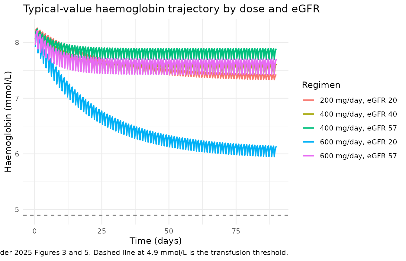
Figure 3 / Figure 5 – HEV viral load decline by dose
The source paper’s Figures 3b/3d show simulated viral load
trajectories on a log scale; the rapid first-phase decline is driven by
the high Imax (= 0.999) and the slow second-phase decay is governed by
the infected-hepatocyte loss rate (kloss = 100 * kdeg).
sim_typical |>
  dplyr::filter(time > 0, virus > 0) |>
  ggplot(aes(time / 24, virus, colour = regimen)) +
  geom_line(linewidth = 0.8) +
  scale_y_log10(labels = scales::label_log()) +
  geom_hline(yintercept = 100, linetype = "dashed", colour = "grey40") +
  labs(
    x = "Time (days)", y = "HEV viral load (IU/mL, log scale)",
    colour = "Regimen",
    title = "Typical-value HEV viral load trajectory by dose and eGFR",
    caption = paste(
      "Replicates the typical-value content of Mulder 2025 Figures 3b/3d.",
      "Dashed line at 100 IU/mL is the clinical \"negative\" threshold."
    )
  ) +
  theme_minimal()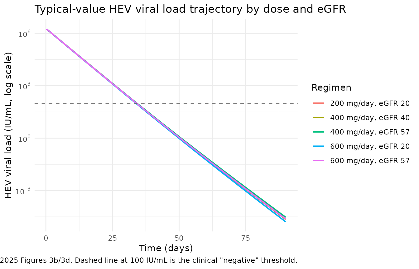
Plasma RBV concentration profile
sim_typical |>
  dplyr::filter(time > 0) |>
  ggplot(aes(time / 24, Cc, colour = regimen)) +
  geom_line(linewidth = 0.8) +
  labs(
    x = "Time (days)", y = "Ribavirin plasma concentration (mg/L)",
    colour = "Regimen",
    title = "Typical-value ribavirin plasma concentration over treatment",
    caption = "Steady-state troughs are reached after ~3-4 weeks; PK alone (not in figures of source paper)."
  ) +
  theme_minimal()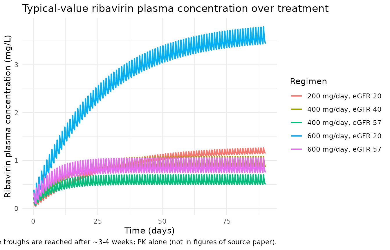
PKNCA validation
The source paper does not tabulate single-dose or steady-state NCA parameters, so this section reports the PKNCA-derived steady-state exposure metrics (Cmax,ss, Cmin,ss, AUC0-tau) that emerge from the typical-value simulation. The values are sanity checks on the PK model rather than a comparison-against-published-NCA exercise. We take steady-state to begin around day 28 (after ~ 4 weeks of daily dosing) and report the metrics over the day-89 to day-90 dosing interval.
# Steady-state window: day 89 to day 90 (= one dosing interval at
# the end of the 90-day course). Restrict the simulation to that
# window and renormalize time so 0 corresponds to the start of the
# interval.
ss_start_h <- (duration_days - 1) * 24
ss_end_h   <- duration_days * 24

sim_pk <- sim_typical |>
  dplyr::filter(!is.na(Cc), time >= ss_start_h, time <= ss_end_h) |>
  dplyr::mutate(time_in_interval = time - ss_start_h) |>
  dplyr::select(id, regimen, time = time_in_interval, Cc) |>
  dplyr::arrange(id, regimen, time) |>
  dplyr::distinct(id, regimen, time, .keep_all = TRUE)

# Dose info for PKNCA (one steady-state dose at time = 0).
dose_pk <- cohorts |>
  dplyr::transmute(id, regimen, time = 0, amt = dose_mg)

conc_obj <- PKNCA::PKNCAconc(sim_pk, Cc ~ time | regimen + id,
                             concu = "mg/L", timeu = "h")
dose_obj <- PKNCA::PKNCAdose(dose_pk, amt ~ time | regimen + id,
                             doseu = "mg")

intervals <- data.frame(
  start    = 0,
  end      = 24,
  cmax     = TRUE,
  cmin     = TRUE,
  tmax     = TRUE,
  auclast  = TRUE,
  cav      = TRUE
)

nca_res <- PKNCA::pk.nca(PKNCA::PKNCAdata(conc_obj, dose_obj, intervals = intervals))
nca_tbl <- as.data.frame(nca_res$result) |>
  dplyr::select(regimen, id, PPTESTCD, PPORRES) |>
  tidyr::pivot_wider(names_from = PPTESTCD, values_from = PPORRES) |>
  dplyr::select(regimen, id,
                dplyr::any_of(c("cmax", "cmin", "tmax", "auclast", "cav")))
knitr::kable(
  nca_tbl, digits = 3,
  caption = paste(
    "Simulated steady-state PKNCA exposure metrics (day 89-90 dosing",
    "interval). The source paper does not tabulate NCA values for",
    "direct comparison; values here are typical-value sanity checks."
  )
)| regimen | id | cmax | cmin | tmax | auclast | cav |
|---|---|---|---|---|---|---|
| 200 mg/day, eGFR 20 | 3 | 1.264 | 1.146 | 6 | 28.604 | 1.192 |
| 400 mg/day, eGFR 40 | 2 | 1.086 | 0.868 | 6 | 22.791 | 0.950 |
| 400 mg/day, eGFR 57 | 5 | 0.703 | 0.500 | 6 | 13.782 | 0.574 |
| 600 mg/day, eGFR 20 | 4 | 3.791 | 3.438 | 6 | 85.813 | 3.576 |
| 600 mg/day, eGFR 57 | 1 | 1.054 | 0.750 | 6 | 20.672 | 0.861 |
Assumptions and deviations
Reference weight 79 kg comes from Wu 2015, not Mulder 2025. Mulder 2025 carries the WT effects on Vc and Vp (exponents 1.29 and 0.725) and the female factor 0.732 on Vp verbatim from the upstream Wu 2015 HCV ribavirin popPK model (reference 19). The centring weight 79 kg is not stated in Mulder 2025; it is taken from Wu 2015 Table 2 (Vc/F = 756 * (WT/79)^1.29). Mulder 2025’s cohort median weight is 74 kg (Table 1) and the per-sex medians used in the source paper’s simulations are 70 kg (male) and 75 kg (female). The choice of 79 kg as the structural reference is therefore an upstream-PK assumption; using 70 or 75 kg would shift the typical volumes by ~ 11-13% (Vc) and ~ 5% (Vp) but would not change the shape of the model output.
-
Linear “inhibitory” slope on kout is encoded as RBV stimulating kout. Mulder 2025 Methods text reads “linear inhibitory effect of RBV on the degradation rate (kout)”. The only encoding that produces the observed haemoglobin decline with increasing RBV exposure (i.e. the central simulation outcome the paper builds its dosing recommendation around) is
kout * (1 + slope * Cc). Encoding the literal sentence as `kout * (1 - slope- Cc)` would give haemoglobin rising with RBV, which contradicts Figures 3a/3c and 5. This extraction therefore interprets the word “inhibitory” as describing the net effect of RBV on haemoglobin (Hb level is suppressed) and not as describing the algebraic sign of the slope on kout (slope is positive, kout is enhanced). This matches the Tod 2005 reference 23 ribavirin-Hb indirect-response formulation cited in the Mulder 2025 Discussion.
Hill coefficient on the sigmoidal-Emax viral inhibition is set to 1. Mulder 2025 Methods describes the IC50 effect of RBV on viral replication as “a sigmoidal Emax model” but Table 2 lists only
Imax(= 0.999, fixed) andIC50(= 1000 ng/L, fixed) – no Hill / gamma exponent is reported. This extraction usesImax * Cc / (Cc + IC50)(Hill = 1) as the basic Emax / Imax form. Because the observed RBV concentrations (0.1-6.2 mg/L = 100-6200 ug/L) are several orders of magnitude above the fixed IC50 (1000 ng/L = 1 ug/L), the inhibition saturates atImaxfor essentially all observed timepoints regardless of the Hill exponent’s exact value; the source paper’s sensitivity analysis on IC50 (Methods, “Viral load”) explicitly notes this insensitivity.-
eGFR cap value (57 mL/min/1.73 m^2) is encoded as fixed. Table 2 reports the cap as an estimated parameter (RSE 0.1%, bootstrap median 57.4, 95% CI 52-180) but the operational role is structural (the centring / capping reference for the eGFR effect on
- and the very low RSE makes the value effectively deterministic. The wide bootstrap CI (52-180) hints at a multimodal distribution – the upper end 180 effectively eliminates the cap because no subject in the cohort has eGFR above 117 – but the point estimate 57 is the most defensible single value for typical-population simulation.
Healthy-hepatocyte half-life (TDEG = 6398 h) and the infected:healthy hepatocyte decay ratio (Factor = 100) come from Dahari 2007 (reference 20). They are not re-estimated by Mulder 2025 and the on-disk source has no other estimate to reconcile.
HEV viral-load residual error model. The source paper reports the residual error as “additive function on the log scale” with SD = 2.01. The vignette encodes this as
vload <- log(virus + 1e-30)withadd(addSd_vload). The 1e-30 floor avoids-Infat the very small numerical-noise floor ofvirus; observed viral loads in the source dataset are always many orders of magnitude above this floor.Per-subject baseline haemoglobin (HGB_BL) and viral load (HEV_VLOAD) are covariates, not estimated parameters. Mulder 2025 sets
kin = kout * HGB_BLper subject so the haemoglobin state is at steady state pre-RBV, and uses the observed baseline viral load directly asvirus(0). For the one subject without an individual baseline haemoglobin, the cohort typical (median) was used (Mulder 2025 Methods). The two covariates are recorded asHGB_BLandHEV_VLOADininst/references/covariate-columns.md; the source-paper column namesHBBASEandVLBASEare recorded as aliases.PKNCA values are NOT compared against a published table because Mulder 2025 does not report NCA parameters. The PKNCA section in this vignette is a sanity check on steady-state PK exposure, not a reproducibility check against the paper.
No NCA validation table. Mulder 2025 reports only graphical PD outputs (Figures 3-5) and a counts-by-Hb-reduction-band table (Supplementary Table S1). No numerical Cmax, Tmax, AUC, or half-life values are given in the manuscript or supplement, so this vignette omits the
ncaComparisonTable()step.