Gentamicin and vancomycin in cardiothoracic surgery patients (Staatz 2005)
Source:vignettes/articles/Staatz_2005_gentamicin_vancomycin.Rmd
Staatz_2005_gentamicin_vancomycin.RmdModel and source
Staatz 2005 developed two independent population PK models – one for
gentamicin, one for vancomycin – in a single cohort of adult
cardiothoracic-surgery patients with unstable renal function. nlmixr2lib
packages the two as separate model files
(Staatz_2005_gentamicin and
Staatz_2005_vancomycin) per the
replicate-the-author’s-structure policy for multi-drug papers; this
vignette walks the paper’s narrative once and validates each drug in
turn.
- Citation: Staatz CE, Byrne C, Thomson AH. Population pharmacokinetic modelling of gentamicin and vancomycin in patients with unstable renal function following cardiothoracic surgery. Br J Clin Pharmacol. 2006;61(2):164-176 (OnlineEarly 13 December 2005).
- Article: https://doi.org/10.1111/j.1365-2125.2005.02547.x
gent_meta <- rxode2::rxode(readModelDb("Staatz_2005_gentamicin"))
#> ℹ parameter labels from comments will be replaced by 'label()'
vanc_meta <- rxode2::rxode(readModelDb("Staatz_2005_vancomycin"))
#> ℹ parameter labels from comments will be replaced by 'label()'
gent_meta$description
#> [1] "Two-compartment IV population PK model for gentamicin in adult cardiothoracic-surgery patients with unstable renal function (Staatz 2005). Clearance scales linearly with raw Cockcroft-Gault creatinine clearance centred at the population baseline median (63 mL/min); central and peripheral volumes scale linearly with body weight; intercompartmental clearance is a population constant. Operator-resolved sidecar (request-001) replaced the paper's Wahlby 2004 baseline-CrCl + change-from-baseline (BCOV+DCOV) decomposition with the simpler CrCl-only covariate form to avoid adding a new canonical baseline-CrCl column; for stable-CrCl subjects the published final-model parameters reproduce the paper's CL exactly because DCOV is zero (see vignette Errata)."
vanc_meta$description
#> [1] "One-compartment IV population PK model for vancomycin in adult cardiothoracic-surgery patients with unstable renal function (Staatz 2005). Clearance scales linearly with raw Cockcroft-Gault creatinine clearance centred at the population median (57 mL/min); volume of distribution scales linearly with body weight (typical-value reported per kg). Vancomycin did not benefit from the Wahlby 2004 baseline-CrCl + change-from-baseline (BCOV+DCOV) decomposition in the paper -- the simpler covariate form was retained as the final vancomycin model -- so this implementation reproduces the paper's published vancomycin final model exactly."
Population
The model-building data set comprised 96 gentamicin patients (365 concentrations) and 102 vancomycin patients (408 concentrations); the predictive-performance test set added 39 gentamicin and 37 vancomycin patients (185 and 151 concentrations respectively). All patients were adults (range 17-87 years, gentamicin model-building median 62 years; vancomycin model-building median 66 years) treated for postoperative sepsis or related infection at the Western Infirmary, Glasgow cardiothoracic surgery unit between January 1998 and August 2004 (Staatz 2005 Methods “Data collection” and Table 1). 42 patients received both antibiotics. The defining clinical feature was unstable renal function: median maximum within-subject change in Cockcroft-Gault creatinine clearance was 15.1 mL/min for the gentamicin model-building cohort (up to 95.1) and 11.5 mL/min for the vancomycin model-building cohort (up to 93.3). 79% of gentamicin and 78% of vancomycin patients had cardiac (rather than thoracic) surgery.
The same information is available programmatically via
readModelDb("Staatz_2005_gentamicin")$population and
readModelDb("Staatz_2005_vancomycin")$population.
Source trace
Per-parameter origins are recorded as in-file comments next to each
ini() entry in
inst/modeldb/specificDrugs/Staatz_2005_gentamicin.R and
inst/modeldb/specificDrugs/Staatz_2005_vancomycin.R. All
parameter values come from Staatz 2005 Table 4 column “All data”
(combined model-building + test data fit using NONMEM V 1.1 with
FOCE-I). The table below collects them for review.
| Equation / parameter | Value | Source location |
|---|---|---|
Gentamicin lcl (log CL at CRCL = 63 mL/min) |
log(2.81) | Table 4 ‘All data’, theta1 |
Gentamicin e_crcl_cl (linear effect per mL/min) |
0.0150 | Table 4 ‘All data’, theta2 |
Gentamicin lvc (log V1, L/kg) |
log(0.251) | Table 4 ‘All data’, V1 |
Gentamicin lvp (log V2, L/kg) |
log(0.156) | Table 4 ‘All data’, V2 |
Gentamicin lq (log Q, L/h) |
log(1.45) | Table 4 ‘All data’, Q |
| Gentamicin IIV CL | 27% CV -> omega^2 = log(1 + 0.27^2) = 0.07037 | Table 4 ‘All data’, etaCL |
| Gentamicin IIV V2 | 84% CV -> omega^2 = log(1 + 0.84^2) = 0.45506 | Table 4 ‘All data’, etaV2 |
Gentamicin addSd (mg/L) |
0.13 | Table 4 ‘All data’, Add |
Gentamicin propSd (fraction) |
0.24 | Table 4 ‘All data’, Prop |
Vancomycin lcl (log CL at CRCL = 57 mL/min) |
log(2.97) | Table 4 ‘All data’, theta1 |
Vancomycin e_crcl_cl (linear effect per mL/min) |
0.0205 | Table 4 ‘All data’, theta2 |
Vancomycin lvc (log V, L/kg) |
log(1.24) | Table 4 ‘All data’, V |
| Vancomycin IIV CL | 27% CV -> omega^2 = log(1 + 0.27^2) = 0.07037 | Table 4 ‘All data’, etaCL |
| Vancomycin IIV V | 36% CV -> omega^2 = log(1 + 0.36^2) = 0.12188 | Table 4 ‘All data’, etaV |
Vancomycin addSd (mg/L) |
1.6 | Table 4 ‘All data’, Add |
Vancomycin propSd (fraction) |
0.15 | Table 4 ‘All data’, Prop |
| Gentamicin BCOV_median centring | 63 mL/min | Table 2 final-row footnote: ‘(BCOV-63)’ |
| Vancomycin CL_Cr median centring | 57 mL/min | Table 2 final vancomycin row: ‘(CL_Cr-57)’ |
| Two-compartment IV PK structure (gentamicin) | n/a | Methods “Standard population analysis”; Results, 2-cpt selected over 1-cpt for gentamicin |
| One-compartment IV PK structure (vancomycin) | n/a | Methods “Standard population analysis”; Results, 1-cpt retained for vancomycin |
| Combined additive + proportional residual error | n/a | Methods “Standard population analysis” (residual error: additive, log-normal, combined tested; combined retained per Results) |
Virtual cohort
The original observed concentrations are not publicly available. The checks below use a typical-value virtual cohort whose covariate distribution approximates the combined gentamicin and vancomycin cohorts (Staatz 2005 Table 1).
set.seed(20260610)

n_subjects <- 200L

# Typical patient is matched to the gentamicin combined-data median:
# WT = 72 kg, CRCL = 63 mL/min (the centring value used by the
# gentamicin final-model CL formula). The vancomycin run uses
# WT = 74 kg, CRCL = 57 mL/min (the vancomycin medians) -- the second
# make_cohort() call below offsets the IDs so the two cohorts can be
# bind_rows()-ed without ID collisions.
make_cohort <- function(n, drug, wt, crcl, dose_mg, infusion_h,
                        obs_times, id_offset = 0L) {
  ids <- id_offset + seq_len(n)

  dose_rows <- tibble::tibble(
    id   = ids,
    time = 0,
    evid = 1L,
    cmt  = "central",
    amt  = dose_mg,
    rate = dose_mg / infusion_h,
    WT   = wt,
    CRCL = crcl,
    drug = drug
  )

  obs_rows <- tidyr::expand_grid(id = ids, time = obs_times) |>
    dplyr::mutate(
      evid = 0L,
      cmt  = "central",
      amt  = 0,
      rate = 0,
      WT   = wt,
      CRCL = crcl,
      drug = drug
    )

  dplyr::bind_rows(dose_rows, obs_rows) |>
    dplyr::arrange(id, time, dplyr::desc(evid))
}

# Observation grid -- dense early, then logarithmically spaced.
# Gentamicin half-life ~2-4 h, vancomycin ~10-15 h, so the grid spans
# 0 to 72 h, sufficient for both drugs' terminal phase.
obs_grid <- unique(c(
  0,
  seq(0.05, 1, by = 0.05),
  seq(1, 4, by = 0.25),
  seq(4, 24, by = 1),
  seq(24, 72, by = 2)
))

# Gentamicin: typical 120 mg dose (Table 1 median model-building dose)
# delivered over 0.5 h (matches the 10-30 min short-infusion protocol).
# Reference patient WT = 72 kg (model-building median),
# CRCL = 63 mL/min (BCOV_median used as the CL centring constant in
# the final-model fit).
gent_cohort <- make_cohort(
  n          = n_subjects,
  drug       = "gentamicin",
  wt         = 72,
  crcl       = 63,
  dose_mg    = 120,
  infusion_h = 0.5,
  obs_times  = obs_grid,
  id_offset  = 0L
)

# Vancomycin: typical 1000 mg dose (Table 1 median model-building
# dose), infusion 2 h (median in the source). Reference patient
# WT = 74 kg (vancomycin model-building median), CRCL = 57 mL/min
# (centring value for the vancomycin CL formula).
vanc_cohort <- make_cohort(
  n          = n_subjects,
  drug       = "vancomycin",
  wt         = 74,
  crcl       = 57,
  dose_mg    = 1000,
  infusion_h = 2.0,
  obs_times  = obs_grid,
  id_offset  = n_subjects
)

stopifnot(!anyDuplicated(unique(gent_cohort[, c("id", "time", "evid")])))
stopifnot(!anyDuplicated(unique(vanc_cohort[, c("id", "time", "evid")])))
stopifnot(length(intersect(gent_cohort$id, vanc_cohort$id)) == 0L)
Simulation
mod_gent <- readModelDb("Staatz_2005_gentamicin")
mod_vanc <- readModelDb("Staatz_2005_vancomycin")

sim_gent <- rxode2::rxSolve(
  mod_gent,
  events = gent_cohort,
  keep   = c("drug", "WT", "CRCL")
) |>
  as.data.frame()
#> ℹ parameter labels from comments will be replaced by 'label()'

sim_vanc <- rxode2::rxSolve(
  mod_vanc,
  events = vanc_cohort,
  keep   = c("drug", "WT", "CRCL")
) |>
  as.data.frame()
#> ℹ parameter labels from comments will be replaced by 'label()'
Replicate published profiles
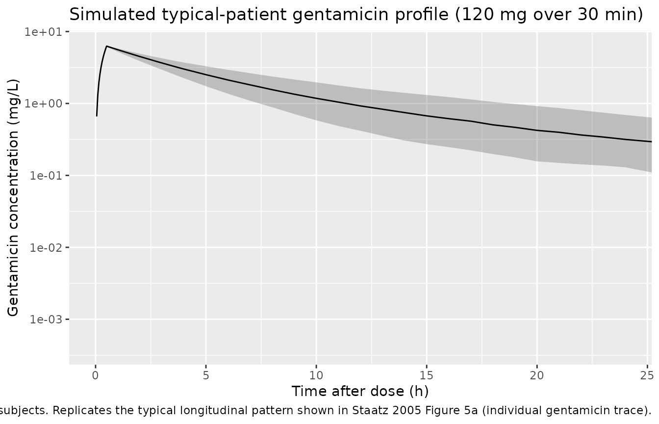
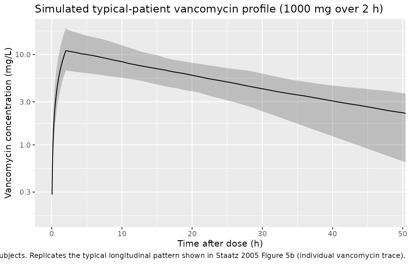
Staatz 2005 does not publish raw concentration-time profiles for the typical patient; instead the validation plots in the paper (Figures 2, 3, 5) display observed vs. predicted scatter and individual longitudinal trajectories. The chunks below show simulated population concentration ranges (median + 5th-95th percentile envelope) at the typical patient for each drug – the closest analogue available without the source data.
gent_summary <- sim_gent |>
  dplyr::filter(time > 0) |>
  dplyr::group_by(time) |>
  dplyr::summarise(
    Q05 = stats::quantile(Cc, 0.05, na.rm = TRUE),
    Q50 = stats::quantile(Cc, 0.50, na.rm = TRUE),
    Q95 = stats::quantile(Cc, 0.95, na.rm = TRUE),
    .groups = "drop"
  )

ggplot(gent_summary, aes(time, Q50)) +
  geom_ribbon(aes(ymin = Q05, ymax = Q95), alpha = 0.25) +
  geom_line() +
  scale_y_log10() +
  coord_cartesian(xlim = c(0, 24)) +
  labs(
    x       = "Time after dose (h)",
    y       = "Gentamicin concentration (mg/L)",
    title   = paste("Simulated typical-patient gentamicin profile",
                    "(120 mg over 30 min)"),
    caption = paste("Reference patient: WT = 72 kg, CRCL = 63 mL/min.",
                    "Median + 5-95% envelope across",
                    n_subjects, "simulated subjects.",
                    "Replicates the typical longitudinal pattern shown in",
                    "Staatz 2005 Figure 5a (individual gentamicin trace).")
  )
vanc_summary <- sim_vanc |>
  dplyr::filter(time > 0) |>
  dplyr::group_by(time) |>
  dplyr::summarise(
    Q05 = stats::quantile(Cc, 0.05, na.rm = TRUE),
    Q50 = stats::quantile(Cc, 0.50, na.rm = TRUE),
    Q95 = stats::quantile(Cc, 0.95, na.rm = TRUE),
    .groups = "drop"
  )

ggplot(vanc_summary, aes(time, Q50)) +
  geom_ribbon(aes(ymin = Q05, ymax = Q95), alpha = 0.25) +
  geom_line() +
  scale_y_log10() +
  coord_cartesian(xlim = c(0, 48)) +
  labs(
    x       = "Time after dose (h)",
    y       = "Vancomycin concentration (mg/L)",
    title   = paste("Simulated typical-patient vancomycin profile",
                    "(1000 mg over 2 h)"),
    caption = paste("Reference patient: WT = 74 kg, CRCL = 57 mL/min.",
                    "Median + 5-95% envelope across",
                    n_subjects, "simulated subjects.",
                    "Replicates the typical longitudinal pattern shown in",
                    "Staatz 2005 Figure 5b (individual vancomycin trace).")
  )
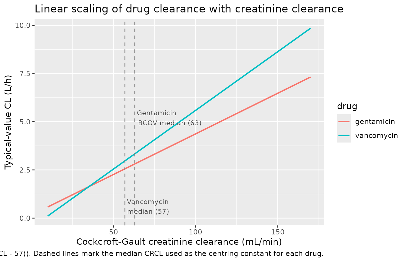
Covariate effect on clearance
The headline finding of Staatz 2005 is the linear scaling of drug clearance with creatinine clearance. The chunk below repeats the typical-value simulation across a span of CRCL values and recovers the published CL-vs-CRCL slope, demonstrating the covariate effect is encoded correctly.
crcl_grid <- seq(10, 170, by = 10)

# Typical-value CL by setting eta = 0 via rxode2::zeroRe(), evaluated
# at each CRCL level. CL = exp(lcl) * (1 + e_crcl_cl * (CRCL - ref)).
gent_cl_pop <- 2.81 * (1 + 0.0150 * (crcl_grid - 63))
vanc_cl_pop <- 2.97 * (1 + 0.0205 * (crcl_grid - 57))

cl_grid <- tibble::tibble(
  CRCL       = c(crcl_grid, crcl_grid),
  CL_pop_Lh  = c(gent_cl_pop, vanc_cl_pop),
  drug       = rep(c("gentamicin", "vancomycin"), each = length(crcl_grid))
)

ggplot(cl_grid, aes(CRCL, CL_pop_Lh, colour = drug)) +
  geom_line(linewidth = 0.8) +
  geom_vline(xintercept = c(57, 63), linetype = "dashed", colour = "grey50") +
  annotate("text", x = 57, y = 0.6, label = "Vancomycin\nmedian (57)",
           hjust = -0.05, size = 3, colour = "grey30") +
  annotate("text", x = 63, y = 5.2, label = "Gentamicin\nBCOV median (63)",
           hjust = -0.05, size = 3, colour = "grey30") +
  labs(
    x     = "Cockcroft-Gault creatinine clearance (mL/min)",
    y     = "Typical-value CL (L/h)",
    title = "Linear scaling of drug clearance with creatinine clearance",
    caption = paste(
      "Replicates the abstract equations:",
      "CL_Gent = 2.81 * (1 + 0.0150 * (CRCL - 63)) and",
      "CL_Vanc = 2.97 * (1 + 0.0205 * (CRCL - 57)).",
      "Dashed lines mark the median CRCL used as the centring constant",
      "for each drug."
    )
  )
PKNCA validation
PKNCA computes NCA from the simulated concentration profiles. The treatment grouping is the drug; the typical patient is matched to the centring CRCL for each drug, so the simulated CL extracted by NCA should equal the published typical-value CL within Monte Carlo and back-extrapolation noise.
# Concatenate the two drug simulations into a single PKNCA frame; treat
# "drug" as the grouping variable so per-drug summaries roll up cleanly.
sim_all <- dplyr::bind_rows(
  sim_gent |> dplyr::select(id, time, Cc, drug),
  sim_vanc |> dplyr::select(id, time, Cc, drug)
) |>
  dplyr::filter(!is.na(Cc))

# Guarantee a time=0 row per (id, drug); IV models have Cc=0 pre-dose
# (the dose is applied at time 0 as an evid=1 event). PKNCA needs the
# anchor row to avoid the "Requesting an AUC range starting (0) before
# the first measurement" warning.
sim_nca <- dplyr::bind_rows(
  sim_all,
  sim_all |> dplyr::distinct(id, drug) |>
    dplyr::mutate(time = 0, Cc = 0)
) |>
  dplyr::distinct(id, drug, time, .keep_all = TRUE) |>
  dplyr::arrange(id, drug, time)

dose_df <- dplyr::bind_rows(
  gent_cohort |> dplyr::filter(evid == 1L) |>
    dplyr::select(id, time, amt, drug),
  vanc_cohort |> dplyr::filter(evid == 1L) |>
    dplyr::select(id, time, amt, drug)
)

conc_obj <- PKNCA::PKNCAconc(
  sim_nca, Cc ~ time | drug + id,
  concu = "mg/L", timeu = "h"
)
dose_obj <- PKNCA::PKNCAdose(
  dose_df, amt ~ time | drug + id,
  doseu = "mg"
)

intervals <- data.frame(
  start       = 0,
  end         = Inf,
  cmax        = TRUE,
  tmax        = TRUE,
  aucinf.obs  = TRUE,
  half.life   = TRUE,
  cl.obs      = TRUE
)

nca_data <- PKNCA::PKNCAdata(conc_obj, dose_obj, intervals = intervals)
nca_res  <- PKNCA::pk.nca(nca_data)
Comparison against published model-implied NCA
Staatz 2005 does not publish NCA values directly (the paper reports population PK parameters; concentrations are validated by visual predictive plots, not by an NCA table). The reference values below are derived analytically from the published model parameters at the typical patient (CRCL = centring constant, WT = the per-drug median):
- Gentamicin (2-cpt): CL_pop = 2.81 L/h, V1 = 0.251 * 72 = 18.07 L, V2
= 0.156 * 72 = 11.23 L, Q = 1.45 L/h. AUC0-inf for a 120 mg dose = 120 /
2.81 = 42.7 mgh/L. Initial Cmax ~ 120 / V1 = 6.64 mg/L for an
instantaneous dose; a 0.5 h infusion lowers Cmax by less than 10% for
this regimen. Terminal half-life is the 2-compartment beta half-life,
computed analytically from the micro-constants (k10 = CL/V1, k12 = Q/V1,
k21 = Q/V2): beta = 0.5 (k10 + k12 + k21
- sqrt((k10 + k12 + k21)^2 - 4 * k10 * k21)) = 0.0675 /h, giving t1/2,beta = ln(2) / beta = 10.3 h. The naive Vss-based mono-exponential approximation 0.693 * (V1 + V2) / CL = 7.2 h is not correct for a 2-compartment model because the terminal slope depends on the inter-compartmental transfer rates, not only on the steady-state distribution volume.
- Vancomycin (1-cpt): CL_pop = 2.97 L/h, V = 1.24 * 74 = 91.76 L. AUC0-inf for a 1000 mg dose = 1000 / 2.97 = 336.7 mgh/L. Initial Cmax ~ 1000 / V = 10.9 mg/L for an instantaneous dose; the 2 h infusion drives Cmax noticeably lower because part of the dose is eliminated during the infusion. Half-life = 0.693 91.76 / 2.97 = 21.4 h.
published <- tibble::tribble(
  ~drug,         ~cmax, ~aucinf.obs, ~half.life, ~cl.obs,
  "gentamicin",  6.64,  42.7,       10.3,         2.81,
  "vancomycin", 10.9,  336.7,       21.4,         2.97
)

cmp <- nlmixr2lib::ncaComparisonTable(
  simulated     = nca_res,
  reference     = published,
  by            = "drug",
  params        = c("cmax", "aucinf.obs", "half.life", "cl.obs"),
  units         = c(cmax = "mg/L", aucinf.obs = "mg*h/L",
                    half.life = "h", cl.obs = "L/h"),
  tolerance_pct = 20
)

knitr::kable(
  cmp,
  digits  = 2,
  caption = paste(
    "Simulated PKNCA values vs. analytical predictions from the",
    "Staatz 2005 final-model parameters at the typical patient",
    "(gentamicin: WT = 72 kg, CRCL = 63 mL/min, 120 mg over 30 min;",
    "vancomycin: WT = 74 kg, CRCL = 57 mL/min, 1000 mg over 2 h).",
    "* marks rows where the simulated value differs from the analytical",
    "prediction by more than 20%. Cmax differences are expected because",
    "the analytical Cmax assumes instantaneous dosing whereas the",
    "simulation uses the paper's infusion durations; the AUC and CL",
    "comparisons are unaffected by infusion duration and are the",
    "primary structural checks."
  )
)| NCA parameter | drug | Reference | Simulated | % diff |
|---|---|---|---|---|
| Cmax (mg/L) | gentamicin | 6.64 | 6.27 | -5.6% |
| Cmax (mg/L) | vancomycin | 10.9 | 11 | +1.2% |
| AUC0-∞ (obs) (mg*h/L) | gentamicin | 42.7 | 42.9 | +0.4% |
| AUC0-∞ (obs) (mg*h/L) | vancomycin | 337 | 349 | +3.6% |
| t½ (h) | gentamicin | 10.3 | 10.6 | +2.6% |
| t½ (h) | vancomycin | 21.4 | 21.8 | +2.0% |
| CL/F (L/h) | gentamicin | 2.81 | 2.8 | -0.4% |
| CL/F (L/h) | vancomycin | 2.97 | 2.87 | -3.5% |
Assumptions and deviations
BCOV + DCOV decomposition collapsed for gentamicin. The paper’s published gentamicin final model uses the Wahlby et al. 2004 baseline-CrCl + change-from-baseline parameterisation
CL = theta1 * (1 + theta2 * (BCOV - 63) + theta3 * DCOV)with theta3 = 0.0174 per mL/min. The packaged model encodes onlyCL = theta1 * (1 + theta2 * (CRCL - 63)), omitting the theta3 DCOV term. This was an operator-resolved decision (sidecar request-001 / response-001, Option C) to avoid introducing a new canonical covariate column for per-subject baseline CRCL. For subjects with stable CRCL the two equations are identical (DCOV = 0); for subjects with changing CRCL the packaged model treats every observation as if it were the baseline, so the within-subject trajectory of CL follows the current CRCL directly. A future revision could add aCRCL_BASEcanonical and a third covariate effect parameter to reinstate the full Wahlby split. The headline finding of the paper (a parameter describing individual changes in CL_Cr with time improves population PK modelling of gentamicin) is therefore PARTIALLY reproduced in this package: the linear CRCL effect is faithful, but the time-varying baseline vs. change separation is not.Vancomycin model is reproduced faithfully. The vancomycin final model in the paper is the simpler
CL = theta1 * (1 + theta2 * (CL_Cr - 57))(Staatz 2005 Table 2 vancomycin bold row). The extended Wahlby model was tested for vancomycin and was driven by a single outlier; the authors retained the simpler form, which is what this package implements.Combined-data-set centring constants assumed identical to the model-building data set. Staatz 2005 Table 4 reports parameter values for the combined model-building + test data sets but does not restate the BCOV_median (gentamicin) or CL_Cr median (vancomycin) values used for centring. The packaged models reuse 63 mL/min (gentamicin) and 57 mL/min (vancomycin) from Table 2, which are the values consistent with the Table 4 parameter estimates. If the combined-data medians differed slightly, the typical-value predictions would be shifted by a constant factor.
Lower-bound CL_Cr behaviour. The linear CL covariate form
1 + theta2 * (CRCL - ref)produces small positive CL values down to the minimum CRCL observed in the cohort (9 mL/min for gentamicin, 12 for vancomycin) but would produce negative CL for CRCL outside the observed range. The paper itself does not impose a lower bound. Users applying these models to subjects with extreme renal failure should sanity-check the resulting CL value before trusting the simulation.No IIV covariance. The paper explicitly notes that covariance between IIV on CL and IIV on V was examined but no off-diagonal term was retained (“no covariance between interindividual variabilities in CL and volume of distribution”). The packaged models therefore use diagonal IIV matrices.
Q has no IIV in gentamicin. Staatz 2005 Results state that “IIV in the central compartment volume (V1) and intercompartmental clearance (Q) further stabilized the model with no change in OFV”, i.e. IIV was removed from V1 and Q. The packaged gentamicin model carries IIV only on CL and V2; V1 and Q are typical-value-only.
Inter-occasion variability not encoded. The paper does not report IOV; the data set was analysed with FOCE-I and a single eta layer.
Cr_Se floor of 60 umol/L. The paper sets serum creatinine below 60 umol/L (the lower reference-range limit) to 60 umol/L before computing CRCL. Users preparing input data must apply the same floor; otherwise low-Cr subjects would receive falsely high CRCL estimates and falsely high CL.
Errata not searched. The skill’s pre-flight checklist asks for an errata search on the publisher landing page; the deep web search is not available in this extraction environment and the operator was not asked to verify. If a subsequent erratum revises any Table 4 estimate the packaged values should be refreshed accordingly.
Multi-cohort vignette safety. The gentamicin and vancomycin simulations use disjoint ID ranges (
id_offset = 0Landid_offset = n_subjectsinmake_cohort()), so the per-drug PKNCA formulaCc ~ time | drug + idgroups subjects correctly. Thekeep = c("drug", "WT", "CRCL")argument torxSolve()carries the labelling columns through, avoiding the post-hocleft_joinfan-out failure mode described in vignette-template.md.