Busulfan (Neroutsos 2022)
Source:vignettes/articles/Neroutsos_2022_busulfan.Rmd
Neroutsos_2022_busulfan.RmdModel and source
- Citation: Neroutsos E, Nalda-Molina R, Paisiou A, Zisaki K, Goussetis E, Spyridonidis A, Kitra V, Grafakos S, Valsami G, Dokoumetzidis A. (2022). Development of a Population Pharmacokinetic Model of Busulfan in Children and Evaluation of Different Sampling Schedules for Precision Dosing. Pharmaceutics 14(3):647. doi:10.3390/pharmaceutics14030647.
- Description: Two-compartment population PK model for intravenous busulfan in children undergoing haematopoietic stem cell transplantation (Neroutsos 2022), with a per-patient syringe-pump infusion lag time supplied as data, allometric body-weight scaling (fixed exponents 0.75 on CL and Q, 1 on V1 and V2) relative to a 70 kg reference, correlated inter-individual variability on CL and V1, three-occasion inter-occasion variability on CL, and a proportional residual error.
- Article: https://doi.org/10.3390/pharmaceutics14030647 (open access)
- Supplement (Table S1 base model, Figure S1, and the NONMEM control script of the final model): https://www.mdpi.com/article/10.3390/pharmaceutics14030647/s1
Neroutsos 2022 fitted a population PK model to intravenous busulfan concentrations from children conditioned for haematopoietic stem cell transplantation in Athens. Small children receive busulfan through a syringe pump at low infusion volumes, and the line dead space delays the drug’s arrival in the circulation by 5-40 min. The authors measured that delay in vitro for each body-weight dosing band and entered it in the dataset as a known lag on the infusion. They then used the model to show that a trapezoidal AUC computed from samples up to 6 h underestimates the true AUC by about 15%, because the last three samples still sit in the distribution phase of a two-compartment profile.
Population
Seventy-six paediatric patients (49 male) were treated at the Bone Marrow Transplantation Unit of the ‘Agia Sofia’ Children’s Hospital of Athens between July 2014 and January 2017 (Neroutsos 2022 Section 2.1 and Table 1). Mean age was 7.6 years (SD 5.1, range 0.5-19) and mean body weight 30.6 kg (SD 21.6, range 7.38-104). Mean CKD-EPI creatinine clearance was 197 mL/min/1.73 m^2. Diagnoses covered malignant and non-malignant indications (acute leukaemias, myelodysplastic syndrome, neuroblastoma, Ewing sarcoma, non-Hodgkin lymphoma, thalassaemia, Blackfan-Diamond anaemia, Wiskott-Aldrich syndrome, adrenoleukodystrophy). Every patient received busulfan (Busilvex) as a 2 h infusion every 6 h for 16 doses, at 0.8-1.2 mg/kg chosen by body-weight band (Table 2). Plasma was sampled before and at 2, 2.5, 4 and 6 h after the start of the first infusion on day 1 and, for most patients, on day 2 (596 samples in total).
The same information is available programmatically via the model’s
population metadata:
pop <- rxode2::rxode(readModelDb("Neroutsos_2022_busulfan"))$population
#> ℹ parameter labels from comments will be replaced by 'label()'
#> Warning: some etas defaulted to non-mu referenced, possible parsing error: etaiov_cl_1, etaiov_cl_2, etaiov_cl_3
#> as a work-around try putting the mu-referenced expression on a simple line
str(pop, max.level = 1)
#> List of 13
#>  $ species       : chr "human"
#>  $ n_subjects    : int 76
#>  $ n_studies     : int 1
#>  $ age_range     : chr "0.5-19 years"
#>  $ age_mean      : chr "7.6 years (SD 5.1)"
#>  $ weight_range  : chr "7.38-104 kg"
#>  $ weight_mean   : chr "30.6 kg (SD 21.6)"
#>  $ sex_female_pct: num 35.5
#>  $ disease_state : chr "Paediatric patients undergoing haematopoietic stem cell (bone marrow) transplantation after busulfan-containing"| __truncated__
#>  $ dose_range    : chr "Intravenous busulfan (Busilvex) 0.8-1.2 mg/kg by body-weight band (Table 2: <9 kg 1 mg/kg; 9-16 kg 1.2; 16-23 k"| __truncated__
#>  $ regions       : chr "Greece ('Agia Sofia' Children's Hospital of Athens, July 2014 - January 2017)."
#>  $ renal_function: chr "CKD-EPI 197 mL/min/1.73 m^2 (SD 41), range 107-346; serum creatinine 0.36 mg/dL (SD 0.15)."
#>  $ notes         : chr "596 plasma busulfan concentrations (HPLC-PDA) sampled at nominal 0, 2, 2.5, 4 and 6 h after the start of the fi"| __truncated__
Source trace
The per-parameter origin is recorded as an in-file comment next to
each ini() entry in
inst/modeldb/specificDrugs/Neroutsos_2022_busulfan.R. The
table below collects them in one place.
| Equation / parameter | Value | Source location |
|---|---|---|
lcl (CL at 70 kg) |
10.7 L/h | Table 3, NONMEM Estimate (RSE 4.05%); abstract |
lvc (V1 at 70 kg) |
39.5 L | Table 3 (RSE 6.84%) |
lq (Q at 70 kg) |
4.68 L/h | Table 3 (RSE 15.2%) |
lvp (V2 at 70 kg) |
17.5 L | Table 3 (RSE 17.2%) |
e_wt_cl_q |
0.75 (fixed) | Supplement control script THETA(5)
(0 0.75) FIX, used on CL and Q; Section 3.2 |
e_wt_vc |
1 (fixed) | Supplement control script THETA(6)
(0 1) FIX, used on V1; Section 3.2 |
| V2 exponent | 1 (hard-coded) | Supplement control script V2=THETA(3)*(BW/70)
|
etalcl, etalvc block |
0.080656, 0.078870, 0.167281 | Table 3 ‘CL IIV’ 0.284, ‘V1 IIV’ 0.409 (SDs), ‘Cor. CL-V1’ 0.679;
control script $OMEGA BLOCK(2)
|
etaiov_cl_1..3 |
0.011025 each | Table 3 ‘CL IOV’ 0.105 (SD); control script
$OMEGA BLOCK(1) then two BLOCK(1) SAME
|
propSd |
0.126 | Table 3 ‘Prop. RE’ (RSE 1.65%); control script
Y=F+F*EPS(1)
|
| Occasion structure |
OCC 1-3 |
Control script
OCC1 = OC1*ETA(3) + OC2*ETA(4) + OC3*ETA(5)
|
| Infusion lag | alag(central) <- T_INFUSION_LAG |
Control script ALAG1=Tlag; Section 2.2; values per band
from Table 2 |
| Structure | 2-compartment, IV | Section 2.2 and 3.1; control script ADVAN3 TRANS4,
S1=V1
|
Virtual cohort
The individual data are not public. The virtual cohort below is built from Table 2: each subject is assigned a body-weight band with probability equal to the band’s share of the 76 patients, a weight drawn log-uniformly over the band’s printed weight range, the band’s mg/kg dose and the band’s infusion lag. Bands whose lag is printed as two values (16-23 kg: 35/25 min; >34 kg: 10/5 min) take either value with equal probability.
set.seed(20220315)
rxode2::rxSetSeed(20220315)

bands <- tibble::tribble(
  ~band,      ~n_pat, ~dose_mgkg, ~wt_lo, ~wt_hi, ~lag1_min, ~lag2_min,
  "<9 kg",         4,       1.00,    7.4,    8.7,       40,        40,
  "9-16 kg",      20,       1.20,    9.2,   15.0,       40,        40,
  "16-23 kg",     13,       1.10,   16.0,   23.0,       35,        25,
  "23-34 kg",     16,       0.95,   25.0,   34.0,       20,        20,
  ">34 kg",       23,       0.80,   34.5,  104.0,       10,         5
)

make_subjects <- function(n, id_offset = 0L) {
  b <- bands[sample(seq_len(nrow(bands)), n, replace = TRUE, prob = bands$n_pat), ]
  tibble(
    id = id_offset + seq_len(n),
    band = factor(b$band, levels = bands$band),
    WT = exp(runif(n, log(b$wt_lo), log(b$wt_hi))),
    dose_mgkg = b$dose_mgkg,
    T_INFUSION_LAG = ifelse(runif(n) < 0.5, b$lag1_min, b$lag2_min) / 60
  )
}

subjects <- make_subjects(200)

# Two days of the q6h regimen (8 doses, 2 h infusions). OCC = 1 on day 1 and
# OCC = 2 on day 2, as in the sampling design (Section 2.1).
make_events <- function(subj, dose_times, obs_times, inf_dur = 2) {
  doses <- tidyr::crossing(subj, time = dose_times) |>
    dplyr::mutate(evid = 1L, amt = dose_mgkg * WT, rate = amt / inf_dur)
  obs <- tidyr::crossing(subj, time = obs_times) |>
    dplyr::mutate(evid = 0L, amt = 0, rate = 0)
  dplyr::bind_rows(doses, obs) |>
    dplyr::mutate(cmt = "central", OCC = ifelse(time < 24, 1L, 2L)) |>
    dplyr::arrange(id, time, dplyr::desc(evid)) |>
    as.data.frame()
}

events <- make_events(
  subjects,
  dose_times = seq(0, 42, by = 6),
  obs_times = sort(unique(c(seq(0, 48, by = 0.25))))
)
stopifnot(!anyDuplicated(events[, c("id", "time", "evid")]))
table(subjects$band)
#>
#>    <9 kg  9-16 kg 16-23 kg 23-34 kg   >34 kg
#>       11       53       24       52       60
Simulation
mod <- readModelDb("Neroutsos_2022_busulfan")
sim <- rxode2::rxSolve(
  mod,
  events = events,
  keep = c("band", "WT", "T_INFUSION_LAG")
) |>
  as.data.frame()
#> ℹ parameter labels from comments will be replaced by 'label()'
#> Warning: some etas defaulted to non-mu referenced, possible parsing error: etaiov_cl_1, etaiov_cl_2, etaiov_cl_3
#> as a work-around try putting the mu-referenced expression on a simple line
stopifnot(!anyNA(sim$Cc))
Replicate published results
Typical-value parameters across the weight range (Section 3.2 and Discussion)
Section 3.2 states that over the observed weight range (7.38-104 kg) the typical CL spans 1.98-14.4 L/h and V1 spans 4.16-58.7 L; the Discussion gives CL 3.4 L/h and V1 8.64 L for a 15.3 kg child. Section 3.2 also reports a terminal half-life of about 3 h at 10 kg and about 5 h above 50 kg.
typ_wt <- c(7.38, 10, 15.3, 50, 70, 104)
ev_typ <- data.frame(
  id = seq_along(typ_wt), time = 0, evid = 0, amt = 0, cmt = "central",
  WT = typ_wt, T_INFUSION_LAG = 0, OCC = 1
)
typ <- rxode2::rxSolve(rxode2::zeroRe(mod), events = ev_typ) |>
  as.data.frame() |>
  dplyr::mutate(
    WT = typ_wt[id],
    beta = 0.5 * ((kel + k12 + k21) - sqrt((kel + k12 + k21)^2 - 4 * kel * k21)),
    thalf = log(2) / beta
  )
#> ℹ parameter labels from comments will be replaced by 'label()'
#> Warning: some etas defaulted to non-mu referenced, possible parsing error: etaiov_cl_1, etaiov_cl_2, etaiov_cl_3
#> as a work-around try putting the mu-referenced expression on a simple line
#> Warning: some etas defaulted to non-mu referenced, possible parsing error: etaiov_cl_1, etaiov_cl_2, etaiov_cl_3
#> as a work-around try putting the mu-referenced expression on a simple line
#> ℹ omega/sigma items treated as zero: 'etalcl', 'etalvc', 'etaiov_cl_1', 'etaiov_cl_2', 'etaiov_cl_3'
#> Warning: multi-subject simulation without without 'omega'

published_typ <- tibble::tribble(
  ~WT,   ~cl_pub, ~vc_pub, ~thalf_pub,
  7.38,     1.98,    4.16,    NA,
  10,         NA,      NA,     3,
  15.3,      3.4,    8.64,    NA,
  50,         NA,      NA,     5,
  104,      14.4,    58.7,    NA
)
typ_cmp <- typ |>
  dplyr::select(WT, cl, vc, thalf) |>
  dplyr::inner_join(published_typ, by = "WT")

typ_cmp |>
  dplyr::rename(
    "Body weight (kg)" = WT,
    "CL model (L/h)" = cl, "CL published (L/h)" = cl_pub,
    "V1 model (L)" = vc, "V1 published (L)" = vc_pub,
    "t1/2 model (h)" = thalf, "t1/2 published (h)" = thalf_pub
  ) |>
knitr::kable(digits = 2, caption = "Typical-value CL, V1 and terminal half-life against the values quoted in Neroutsos 2022.")| Body weight (kg) | CL model (L/h) | V1 model (L) | t1/2 model (h) | CL published (L/h) | V1 published (L) | t1/2 published (h) |
|---|---|---|---|---|---|---|
| 7.38 | 1.98 | 4.16 | 2.82 | 1.98 | 4.16 | NA |
| 10.00 | 2.49 | 5.64 | 3.04 | NA | NA | 3 |
| 15.30 | 3.42 | 8.63 | 3.38 | 3.40 | 8.64 | NA |
| 50.00 | 8.31 | 28.21 | 4.54 | NA | NA | 5 |
| 104.00 | 14.40 | 58.69 | 5.46 | 14.40 | 58.70 | NA |
# Same parameters on both sides (Table 3 values vs the paper's own derived
# numbers), so only rounding separates them.
chk_cl <- dplyr::filter(typ_cmp, !is.na(cl_pub))
stopifnot(
  max(abs(chk_cl$cl / chk_cl$cl_pub - 1)) < 0.02,
  max(abs(chk_cl$vc / chk_cl$vc_pub - 1)) < 0.02
)
# 'about 3 h' and 'near 5 h' are rounded statements.
chk_th <- dplyr::filter(typ_cmp, !is.na(thalf_pub))
stopifnot(max(abs(chk_th$thalf - chk_th$thalf_pub)) < 0.5)
The paper also reports a mean terminal half-life of about 4 h (CV 22%) across all its patients. Over the virtual cohort (weights drawn from Table 2, with between-subject variability on CL and V1):
indiv <- sim |>
  dplyr::filter(time == 0) |>
  dplyr::mutate(
    beta = 0.5 * ((kel + k12 + k21) - sqrt((kel + k12 + k21)^2 - 4 * kel * k21)),
    thalf = log(2) / beta
  )
thalf_summary <- c(
  mean = mean(indiv$thalf),
  cv_pct = 100 * sd(indiv$thalf) / mean(indiv$thalf)
)
round(thalf_summary, 2)
#>   mean cv_pct
#>   3.99  24.73
# Centre of the distribution against the published 'about 4 h'; the CV is
# reported for comparison with the published 22% but not gated (it depends on
# the weight mix of the virtual cohort).
stopifnot(abs(median(indiv$thalf) - 4) < 0.75)
Concentration-time profiles (Figure 2)
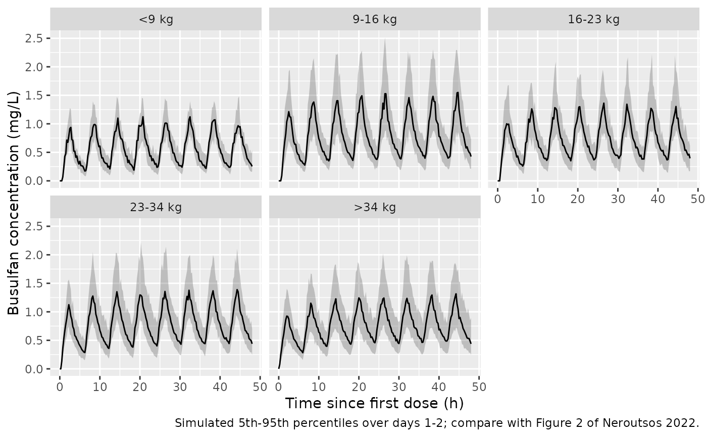
Figure 2 of the paper is a prediction-corrected VPC against time after dose. The plot below shows the 5th, 50th and 95th percentiles of the simulated concentrations, with residual error, over the first two days of dosing, split by weight band. The infusion lag is visible as the delayed rise in the lighter bands.
sim |>
  dplyr::filter(time <= 48) |>
  dplyr::group_by(band, time) |>
  dplyr::summarise(
    Q05 = quantile(sim, 0.05),
    Q50 = quantile(sim, 0.50),
    Q95 = quantile(sim, 0.95),
    .groups = "drop"
  ) |>
  ggplot(aes(time, Q50)) +
  geom_ribbon(aes(ymin = Q05, ymax = Q95), alpha = 0.25) +
  geom_line() +
  facet_wrap(~band) +
  labs(
    x = "Time since first dose (h)",
    y = "Busulfan concentration (mg/L)",
    caption = "Simulated 5th-95th percentiles over days 1-2; compare with Figure 2 of Neroutsos 2022."
  )
Exposure against the therapeutic range (Section 3.3)
The busulfan label targets a per-dose AUC of 900-1500 uM x min. Using the Bayesian clearance estimates of the real patients, Neroutsos 2022 found 19% below, 58.9% within and 21.9% above that range. The per-dose AUC of the virtual cohort at the first occasion is dose / CL (busulfan molar mass 246.3 g/mol).
mw <- 246.3
tr <- indiv |>
  dplyr::left_join(dplyr::select(subjects, id, dose_mgkg), by = "id") |>
  dplyr::mutate(
    auc_umolmin = (dose_mgkg * WT / cl) / mw * 1000 * 60,
    category = cut(auc_umolmin, c(-Inf, 900, 1500, Inf),
                   labels = c("below", "within", "above"))
  )
tr_tab <- tibble::tibble(
  category = c("below", "within", "above"),
  simulated_pct = as.numeric(100 * prop.table(table(tr$category))),
  published_pct = c(19, 58.9, 21.9)
)
tr_tab |>
  dplyr::rename(
    "AUC vs 900-1500 uM x min" = category,
    "Simulated (%)" = simulated_pct,
    "Published, Bayesian AUC (%)" = published_pct
  ) |>
knitr::kable(digits = 1, caption = "Share of patients below, within and above the therapeutic range after the first dose.")| AUC vs 900-1500 uM x min | Simulated (%) | Published, Bayesian AUC (%) |
|---|---|---|
| below | 14.5 | 19.0 |
| within | 66.5 | 58.9 |
| above | 19.0 | 21.9 |
PKNCA validation: trapezoidal AUC against the true AUC (Figure 3)
Neroutsos 2022 simulated 1000 patients under three sampling schedules and compared a trapezoidal AUC (log-linear rule, terminal slope from the last three samples) with the true AUC = dose / CL. Schedules 1 (2.5, 3, 4, 6 h) and 2 (2.5, 4, 6 h) follow the first dose of the q6h regimen. Schedule 3 (3, 6, 9, 12 h) follows a once-daily 3 h infusion of four times the q6h dose, for which the lag is negligible. Figure 3 of the paper shows, for the trapezoidal AUC, a bias of about 0.155, 0.143 and 0.027 and an imprecision of about 0.205, 0.192 and 0.095 for Schedules 1, 2 and 3 (read from the bar chart by the maintainers; the values are on the fractional scale, relative to the true AUC).
The PKNCA calculation below reproduces that exercise on the virtual cohort. It uses observations with residual error at the schedule times, and times measured from the actual start of drug entry (the dose time plus the known lag).
sch_qid <- make_events(subjects, dose_times = 0, obs_times = c(2.5, 3, 4, 6)) |>
  dplyr::mutate(OCC = 1L)
sim_qid <- rxode2::rxSolve(mod, events = sch_qid, keep = c("band", "T_INFUSION_LAG")) |>
  as.data.frame()

sch_qd <- subjects |>
  dplyr::mutate(dose_mgkg = 4 * dose_mgkg, T_INFUSION_LAG = 0) |>
  make_events(dose_times = 0, obs_times = c(3, 6, 9, 12), inf_dur = 3) |>
  dplyr::mutate(OCC = 1L)
sim_qd <- rxode2::rxSolve(mod, events = sch_qd, keep = c("band", "T_INFUSION_LAG")) |>
  as.data.frame()

sparse <- dplyr::bind_rows(
  sim_qid |> dplyr::mutate(schedule = "Schedule 1"),
  sim_qid |> dplyr::filter(time != 3) |> dplyr::mutate(schedule = "Schedule 2"),
  sim_qd |> dplyr::mutate(schedule = "Schedule 3")
) |>
  dplyr::mutate(time = time - T_INFUSION_LAG, Cc = sim) |>
  dplyr::select(id, schedule, time, Cc, cl)

# True AUC per subject and schedule (dose / individual CL).
dose_df <- dplyr::bind_rows(
  sch_qid |> dplyr::filter(evid == 1) |> dplyr::mutate(schedule = "Schedule 1"),
  sch_qid |> dplyr::filter(evid == 1) |> dplyr::mutate(schedule = "Schedule 2"),
  sch_qd |> dplyr::filter(evid == 1) |> dplyr::mutate(schedule = "Schedule 3")
) |>
  dplyr::select(id, schedule, time, amt)

truth <- sparse |>
  dplyr::distinct(id, schedule, cl) |>
  dplyr::left_join(dose_df, by = c("id", "schedule")) |>
  dplyr::mutate(auc_true = amt / cl)

# Pre-dose record at the start of drug entry, then PKNCA with the terminal
# slope forced onto the last three samples.
conc_nca <- dplyr::bind_rows(
  sparse,
  sparse |> dplyr::distinct(id, schedule) |> dplyr::mutate(time = 0, Cc = 0)
) |>
  dplyr::filter(!is.na(Cc)) |>
  dplyr::distinct(id, schedule, time, .keep_all = TRUE) |>
  dplyr::arrange(schedule, id, time) |>
  dplyr::group_by(schedule, id) |>
  dplyr::mutate(last3 = dplyr::row_number() > dplyr::n() - 3) |>
  dplyr::ungroup()

conc_obj <- PKNCA::PKNCAconc(
  conc_nca, Cc ~ time | schedule + id,
  include_half.life = "last3"
)
dose_obj <- PKNCA::PKNCAdose(dose_df, amt ~ time | schedule + id)
intervals <- data.frame(start = 0, end = Inf, aucinf.obs = TRUE, cmax = TRUE)
nca_res <- PKNCA::pk.nca(PKNCA::PKNCAdata(
  conc_obj, dose_obj,
  intervals = intervals,
  options = list(auc.method = "lin up/log down")
))
include_half.life fixes the terminal-slope points to the
last three samples of each profile, as in Section 3.4 of the paper,
instead of letting PKNCA choose them by adjusted r-squared.
auc_trap <- as.data.frame(nca_res) |>
  dplyr::filter(PPTESTCD == "aucinf.obs") |>
  dplyr::select(id, schedule, auc_trap = PPORRES)

perf <- truth |>
  dplyr::inner_join(auc_trap, by = c("id", "schedule")) |>
  dplyr::filter(!is.na(auc_trap)) |>
  dplyr::mutate(rel_err = (auc_true - auc_trap) / auc_true) |>
  dplyr::group_by(schedule) |>
  dplyr::summarise(
    n = dplyr::n(),
    bias = mean(rel_err),
    imprecision = sqrt(mean(rel_err^2)),
    .groups = "drop"
  ) |>
  dplyr::left_join(
    tibble::tibble(
      schedule = c("Schedule 1", "Schedule 2", "Schedule 3"),
      bias_pub = c(0.155, 0.143, 0.027),
      imprecision_pub = c(0.205, 0.192, 0.095)
    ),
    by = "schedule"
  )

perf |>
  dplyr::rename(
    "Schedule" = schedule, "Subjects" = n,
    "Bias (sim)" = bias, "Bias (Figure 3)" = bias_pub,
    "Imprecision (sim)" = imprecision, "Imprecision (Figure 3)" = imprecision_pub
  ) |>
knitr::kable(digits = 3, caption = "Trapezoidal AUC relative to the true AUC: bias = mean((true - trap) / true), imprecision = root-mean-square of the same relative error.")| Schedule | Subjects | Bias (sim) | Imprecision (sim) | Bias (Figure 3) | Imprecision (Figure 3) |
|---|---|---|---|---|---|
| Schedule 1 | 200 | 0.158 | 0.202 | 0.155 | 0.205 |
| Schedule 2 | 200 | 0.174 | 0.198 | 0.143 | 0.192 |
| Schedule 3 | 200 | 0.056 | 0.098 | 0.027 | 0.095 |
ggplot(
  perf |>
    dplyr::select(schedule, Simulated = bias, `Figure 3` = bias_pub) |>
    tidyr::pivot_longer(-schedule, names_to = "source", values_to = "bias"),
  aes(schedule, bias, fill = source)
) +
  geom_col(position = "dodge") +
  labs(x = NULL, y = "Bias of trapezoidal AUC (fraction)", fill = NULL,
       caption = "Replicates the trapezoidal-AUC bars of Figure 3 of Neroutsos 2022.")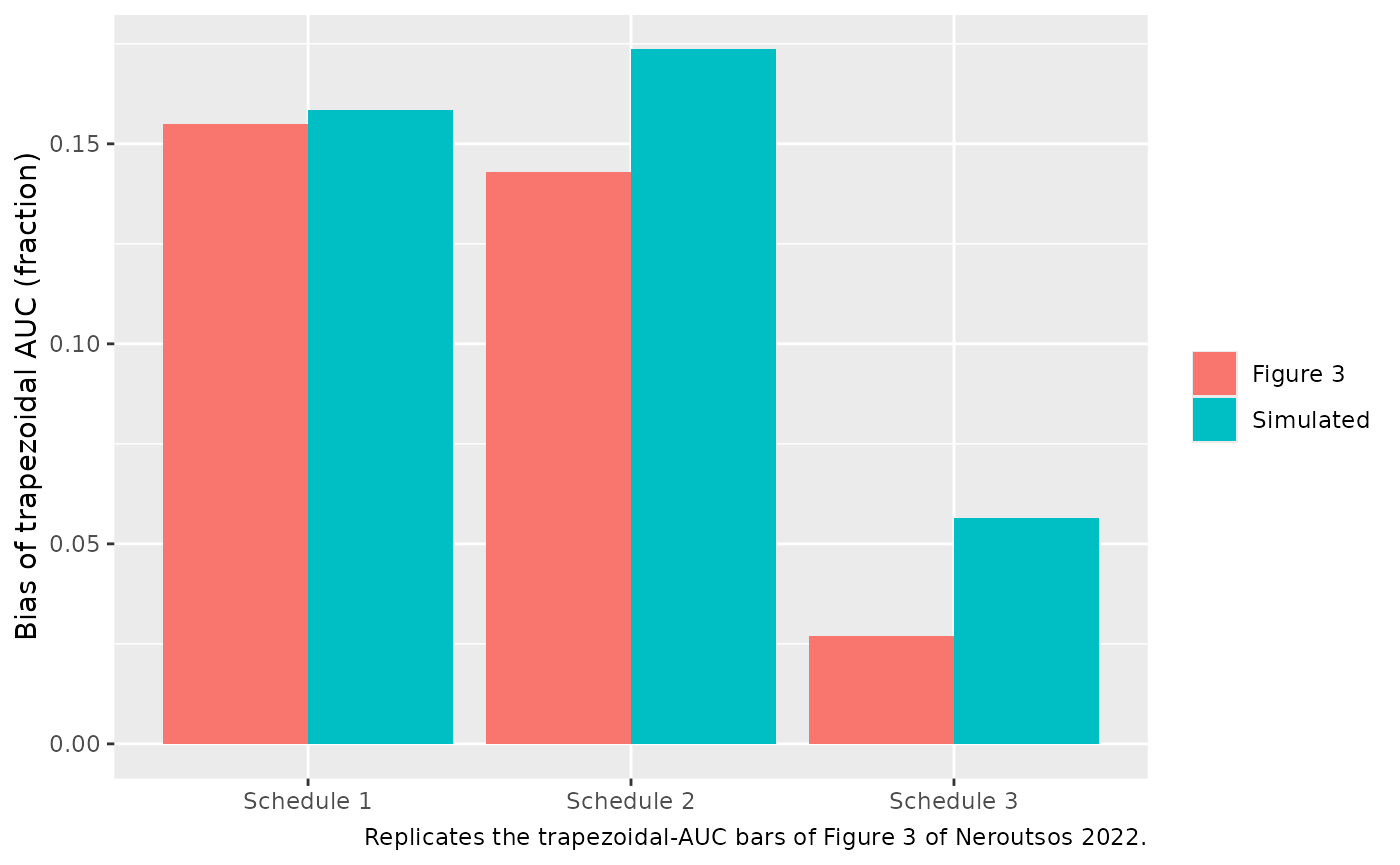
The six-hour schedules underestimate the true AUC because the last three samples still include the distribution phase, so the terminal slope is too steep. The 12 h schedule reaches the terminal phase and is nearly unbiased. Those are the paper’s findings, and both follow from the two-compartment disposition parameters. Schedules 1 and 2 land close to the published bars. For Schedule 3 the simulated bias comes out around twice the published 0.027, though still small next to the 6 h schedules. The paper does not print the details of its trapezoidal calculation (see “Assumptions and deviations”), so the gate below checks only that the 12 h schedule removes most of the bias.
b <- setNames(perf$bias, perf$schedule)
stopifnot(
  # Sampling to 6 h: a clear underestimate of roughly the published size.
  b[["Schedule 1"]] > 0.08, b[["Schedule 1"]] < 0.25,
  b[["Schedule 2"]] > 0.08, b[["Schedule 2"]] < 0.25,
  # Sampling to 12 h: much smaller bias.
  abs(b[["Schedule 3"]]) < 0.08
)
The Bayesian (model-based) AUC bars of Figure 3 need a posthoc estimation step for every simulated patient and are not reproduced here.
Assumptions and deviations
- Covariate cohort. The paper sampled covariates from its own dataset, which is not public. The virtual cohort is built from Table 2 (band shares, per-band weight ranges, doses and lags). The weight range printed for the 16-23 kg band (16.0-66.7 kg) cannot be right for that band; the virtual cohort draws 16-23 kg.
-
Two-valued lag bands. Table 2 gives the lag for the
16-23 kg band as ‘35/25’ min and for the >34 kg band as ‘10/5’ min
without saying which patients received which value. The virtual cohort
assigns each value with probability 0.5. Users with patient-level
information should supply the actual lag in
T_INFUSION_LAG(in hours). -
Scale of the random effects. Table 3 reports the
IIV, IOV and residual error as standard deviations (the abstract’s 28%
and 41% for CL and V1 IIV and 11% for CL IOV match 0.284, 0.409 and
0.105). The model’s variances are their squares, and the CL-V1
covariance is 0.679 x 0.284 x 0.409. The initial estimates in the
supplement control script
(
$OMEGA BLOCK(2) 0.0697 0.0662 0.106, IOV 0.0125,$SIGMA 0.0136) are on the same scale. -
Occasions. The control script assigns separate IOV
etas to occasions 1-3. It also builds an unused
OC4indicator, so occasion 4 has no IOV. The paper does not define the occasions beyond sampling on day 1 and, for most patients, day 2. The simulations use occasion 1 for day 1 and occasion 2 for day 2. -
Concentration units. The paper does not print the
concentration unit. With doses in mg and
S1 = V1in litres, the model predicts mg/L. The resulting first-dose AUCs fall within the 900-1500 uM x min target range, which supports that reading. - Trapezoidal method. The paper cites its own earlier work for the trapezoidal method with the lag and does not print the details. Here the sample times are shifted by the known lag and a zero pre-dose concentration is placed at the start of drug entry. The half-life uses the last three samples, as in Section 3.4.
- Figure 3 values were read from the bar chart by the maintainers, so they carry roughly +/-0.005 reading uncertainty.
- Typographical issues in the source, none of which affect the model: Table 3’s bootstrap CI for CL is printed as ‘9.79-1.47’ (presumably 9.79-11.47); Table 1’s height range ‘0.71-207’ cm is implausible; and the Section 3.2 equation for V1 is printed with the typical value on both sides. No correction notice for the article was found as of 2026-09-30.