Gepotidacin (Nguyen 2022) • nlmixr2lib

Model and source

Citation: Nguyen D, Shaik JS, Tai G, Tiffany C, Perry C, Dumont E, Gardiner D, Barth A, Singh R, Hossain M. Comparison between physiologically based pharmacokinetic and population pharmacokinetic modelling to select paediatric doses of gepotidacin in plague. Br J Clin Pharmacol. 2022;88(2):416-428. doi:10.1111/bcp.14996
Description: Three-compartment intravenous population PK model for gepotidacin in healthy adults and adults with acute bacterial skin and skin structure infections, with allometric body-weight scaling of every clearance and volume and an estimated (modelled) infusion duration; extended to paediatric dose selection for plague by a fixed paracetamol-derived postmenstrual-age maturation function on clearance applied below 2 years of age. The paper’s Simcyp whole-body PBPK model is not included.
Article: https://doi.org/10.1111/bcp.14996 (open access, PMC9293063)
Supplement: Supporting Information (bcp14996-sup-0001), which holds the final population PK parameter table (Table S2) and the paediatric exposure figures (Figures S12 and S13).

Nguyen et al. compared a Simcyp whole-body PBPK model with a NONMEM population PK model to select paediatric intravenous doses of gepotidacin for plague under the FDA Animal Rule. Only the population PK model is packaged here. The PBPK model depends on the Simcyp platform’s built-in physiology and CYP3A4 / GFR ontogeny, none of which is printed in the paper.

Population

The population PK model was fitted to 249 adults: 140 healthy volunteers from four phase I studies (single 1-h infusions of 200-1800 mg, a single 2-h infusion of 1800 mg, and repeat 2-h infusions of 400-1000 mg twice daily or 1000 mg three times daily, including a Japanese cohort) and 109 patients with acute bacterial skin and skin structure infections (ABSSSI) from the phase II study BTZ116704 (750 or 1000 mg twice daily, or 1000 mg three times daily, for up to 10 days). Study mean ages ranged from 26.6 to 44.7 years (Table 1). The paper reports no weight range, sex split or race distribution for the fitted dataset. Healthy subjects and ABSSSI patients had the same PK.

For the paediatric dose selection the authors added a maturation function on clearance, with constants fixed from a published paracetamol model, and simulated four weight cohorts of 100 children each, aged 0.01-19.6 years and weighing 2.5-79 kg.

The same information is available programmatically via readModelDb("Nguyen_2022_gepotidacin")()$population.

Source trace

Equation / parameter	Value	Source location
`lcl` (CL, 70 kg)	log(38.0) L/h	Table S2
`lvc` (V1, 70 kg)	log(20.1) L	Table S2
`lq` (Q2, 70 kg)	log(3.85) L/h	Table S2
`lvp` (V2, 70 kg)	log(67.1) L	Table S2
`lq2` (Q3, 70 kg)	log(48.5) L/h	Table S2
`lvp2` (V3, 70 kg)	log(70.3) L	Table S2
`ld1_inf1h` (D1, 1-h infusion)	log(1.06) h	Table S2
`ld1_inf2h` (D1, 2-h infusion)	log(2.14) h	Table S2
`e_wt_cl`	0.75 (fixed)	Table S2 footnote; Section 2.2
`e_wt_vc_q_vp_q2_vp2`	1 (fixed)	Table S2 footnote
`pma_tm50`	52.2 weeks (fixed)	Section 2.2.2
`pma_hill`	3.43 (fixed)	Section 2.2.2
`etalcl`	0.0302 (17.5 CV%)	Table S2
`etalvc`	0.3727 (67.2 CV%)	Table S2
`etalq`	0.1792 (44.3 CV%)	Table S2
`etalvp`	0.1554 (41.0 CV%)	Table S2
`etalq2`	0.0578 (24.4 CV%)	Table S2
`etalvp2`	0.0098 (9.92 CV%)	Table S2
`propSd`	0.222	Table S2, ‘Residual Error’ (CV% of proportional error)
Three-compartment structure, IV input to central	n/a	Section 2.2
`CL = 38.0 * (WT/70)^0.75`; `V1, Q2, V2, Q3, V3` linear in `WT/70`	n/a	Table S2 footnote
`FMAT = PMA^Hill / (TM50^Hill + PMA^Hill)` on CL, below 2 years only	n/a	Section 2.2.2 equation and text
`PMA (weeks) = PNA (weeks) + 40` (full-term birth)	n/a	Section 2.2.2

The variances are log(1 + CV^2). That conversion is one of the assumptions listed at the end of this article.

Virtual cohorts

Original observed data are not publicly available. Three virtual cohorts are built below.

rxode2::rxSetSeed(20220202)
set.seed(20220202)

# Dose and observation records for one subject set. Every dose record carries
# rate = -2 so that rxode2 uses the model's modelled infusion duration
# dur(central); TINF selects which estimated D1 applies.
make_events <- function(subj, dose_times, tinf, obs_times) {
  doses <- tidyr::expand_grid(subj, time = dose_times) |>
    dplyr::mutate(evid = 1L, amt = .data$dose_mg, rate = -2, TINF = tinf)
  obs <- tidyr::expand_grid(subj, time = obs_times) |>
    dplyr::mutate(evid = 0L, amt = 0, rate = 0, TINF = tinf)
  dplyr::bind_rows(doses, obs) |>
    dplyr::mutate(cmt = "central") |>
    dplyr::arrange(.data$id, .data$time, dplyr::desc(.data$evid)) |>
    dplyr::select("id", "time", "evid", "amt", "rate", "cmt", "WT", "PNA", "TINF", "cohort")
}

# Adult body weights: log-normal around 78 kg, truncated to the 49.5-117.9 kg
# range of the paper's adult simulation dataset (Section 2.2.1).
draw_adult_wt <- function(n) {
  wt <- exp(rnorm(n * 3, log(78), 0.2))
  wt <- wt[wt >= 49.5 & wt <= 117.9]
  wt[seq_len(n)]
}

Adults at steady state (Section 2.2.1)

200 adults aged 18-71 years receive 1000 mg every 8 hours as a 2-hour infusion for 10 days, which is the regimen the FDA Animal Rule supports. The dosing interval at steady state is the last one, 216-224 h.

tau <- 8
n_adult <- 200
adult_subj <- tibble::tibble(
  id = seq_len(n_adult),
  WT = draw_adult_wt(n_adult),
  PNA = 12 * runif(n_adult, 18, 71),
  dose_mg = 1000,
  cohort = "Adult 1000 mg TID"
)
dose_times_ss <- seq(0, by = tau, length.out = 28)
obs_ss <- sort(unique(c(seq(0, 216, by = 2), 216 + c(0, 0.5, 1, 1.5, 2, 2.1, 2.25, 2.5, 3, 4, 5, 6, 7, 8))))
events_ss <- make_events(adult_subj, dose_times_ss, tinf = 2, obs_times = obs_ss)

Adults after a single dose (Table 3)

Table 3 compares single 2-hour infusions of 400, 750, 1000 and 1800 mg and a single 3-hour infusion of 1500 mg. Each arm has 100 adults.

sd_arms <- tibble::tribble(
  ~cohort, ~dose_mg, ~tinf,
  "400 mg (SD)", 400, 2,
  "750 mg (SD)", 750, 2,
  "1000 mg (SD)", 1000, 2,
  "1500 mg (SD, 3-h)", 1500, 3,
  "1800 mg (SD)", 1800, 2
)
n_sd <- 100
obs_sd <- sort(unique(c(0, 0.5, 1, 1.5, 2, 2.14, 2.5, 3, 3.1, 3.5, 4, 5, 6, 8, 10, 12, 16, 24, 36, 48, 72)))
events_sd <- dplyr::bind_rows(lapply(seq_len(nrow(sd_arms)), function(i) {
  subj <- tibble::tibble(
    id = 1000L + (i - 1L) * n_sd + seq_len(n_sd),
    WT = draw_adult_wt(n_sd),
    PNA = 12 * runif(n_sd, 18, 55),
    dose_mg = sd_arms$dose_mg[i],
    cohort = sd_arms$cohort[i]
  )
  make_events(subj, 0, tinf = sd_arms$tinf[i], obs_times = obs_sd)
}))
stopifnot(!anyDuplicated(unique(events_sd[, c("id", "time", "evid")])))

Children (Section 2.2.2, Figures S12 and S13)

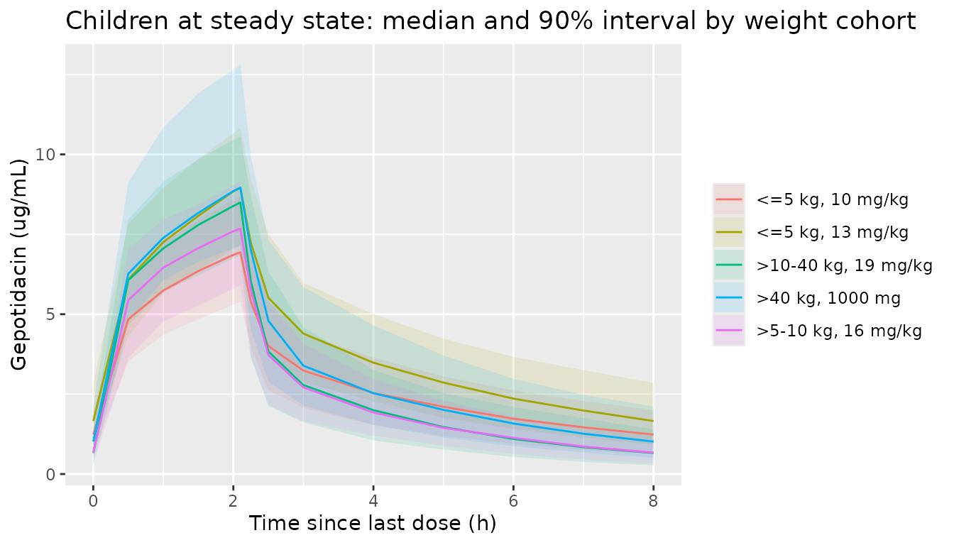
The paper built its paediatric dataset from CDC and WHO growth charts. Here ages are drawn uniformly within each age bracket of Table 2, and weights come from an approximate median weight-for-age curve with 12% log-normal spread. Subjects whose weight falls outside the cohort’s weight bracket are redrawn. Every child receives 2-hour infusions every 8 hours for 10 days. Doses are 10 mg/kg for 5 kg and under (the final PopPK dose; 13 mg/kg is also simulated), 16 mg/kg above 5 kg up to 10 kg, 19 mg/kg above 10 kg up to 40 kg, and a fixed 1000 mg above 40 kg.

# Approximate median weight-for-age (WHO under 2 years, CDC above), age in months.
wfa_age <- c(0, 1, 3, 6, 12, 24, 60, 120, 168, 216, 240)
wfa_wt <- c(3.3, 4.4, 6.1, 7.7, 9.6, 12.2, 18.3, 31.9, 50.0, 65.0, 70.0)
median_wt <- function(pna) exp(approx(wfa_age, log(wfa_wt), xout = pna, rule = 2)$y)

paed_cohorts <- tibble::tribble(
  ~cohort, ~age_lo, ~age_hi, ~wt_lo, ~wt_hi, ~mgkg, ~fixed_mg,
  "<=5 kg, 10 mg/kg", 0.12, 3, 0, 5, 10, NA,
  "<=5 kg, 13 mg/kg", 0.12, 3, 0, 5, 13, NA,
  ">5-10 kg, 16 mg/kg", 3, 12, 5, 10, 16, NA,
  ">10-40 kg, 19 mg/kg", 12, 168, 10, 40, 19, NA,
  ">40 kg, 1000 mg", 168, 235, 40, 200, NA, 1000
)
draw_paed <- function(n, age_lo, age_hi, wt_lo, wt_hi) {
  out <- tibble::tibble(PNA = numeric(0), WT = numeric(0))
  while (nrow(out) < n) {
    pna <- runif(4 * n, age_lo, age_hi)
    wt <- median_wt(pna) * exp(rnorm(4 * n, 0, 0.12))
    keep <- wt > wt_lo & wt <= wt_hi
    out <- dplyr::bind_rows(out, tibble::tibble(PNA = pna[keep], WT = wt[keep]))
  }
  out[seq_len(n), ]
}
n_paed <- 100
events_paed <- dplyr::bind_rows(lapply(seq_len(nrow(paed_cohorts)), function(i) {
  pc <- paed_cohorts[i, ]
  subj <- draw_paed(n_paed, pc$age_lo, pc$age_hi, pc$wt_lo, pc$wt_hi) |>
    dplyr::mutate(
      id = 5000L + (i - 1L) * n_paed + dplyr::row_number(),
      dose_mg = if (is.na(pc$fixed_mg)) pc$mgkg * .data$WT else pc$fixed_mg,
      cohort = pc$cohort
    )
  make_events(subj, dose_times_ss, tinf = 2, obs_times = obs_ss)
}))
stopifnot(!anyDuplicated(unique(events_paed[, c("id", "time", "evid")])))

Simulation

mod <- readModelDb("Nguyen_2022_gepotidacin")
sim_ss <- rxode2::rxSolve(mod, events = events_ss, keep = "cohort")
#> ℹ parameter labels from comments will be replaced by 'label()'
sim_sd <- rxode2::rxSolve(mod, events = events_sd, keep = "cohort")
sim_paed <- rxode2::rxSolve(mod, events = events_paed, keep = c("cohort", "WT", "PNA"))
stopifnot(
  !anyNA(sim_ss$Cc), !anyNA(sim_sd$Cc), !anyNA(sim_paed$Cc)
)

Concentration-time profiles

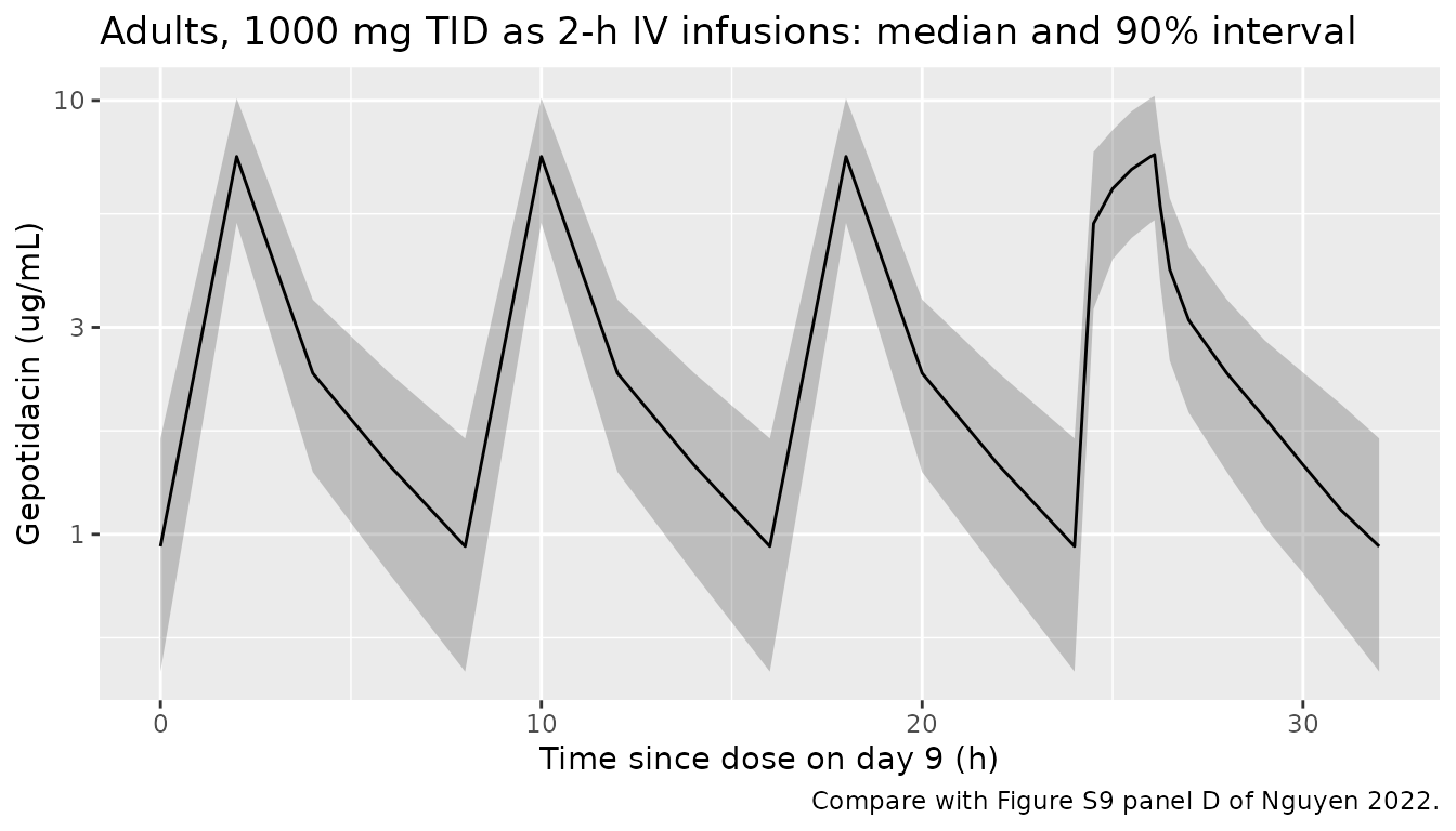
The adult steady-state profile below has the same regimen as the VPC panel D of Figure S9 (1000 mg IV every 8 hours as a 2-hour infusion).

sim_ss |>
  dplyr::filter(time >= 192) |>
  dplyr::group_by(time) |>
  dplyr::summarise(
    Q05 = quantile(Cc, 0.05), Q50 = median(Cc), Q95 = quantile(Cc, 0.95),
    .groups = "drop"
  ) |>
  ggplot(aes(time - 192, Q50)) +
  geom_ribbon(aes(ymin = Q05, ymax = Q95), alpha = 0.25) +
  geom_line() +
  scale_y_log10() +
  labs(
    x = "Time since dose on day 9 (h)", y = "Gepotidacin (ug/mL)",
    title = "Adults, 1000 mg TID as 2-h IV infusions: median and 90% interval",
    caption = "Compare with Figure S9 panel D of Nguyen 2022."
  )

sim_paed |>
  dplyr::filter(time >= 216) |>
  dplyr::group_by(cohort, time) |>
  dplyr::summarise(Q50 = median(Cc), Q05 = quantile(Cc, 0.05), Q95 = quantile(Cc, 0.95), .groups = "drop") |>
  ggplot(aes(time - 216, Q50, colour = cohort, fill = cohort)) +
  geom_ribbon(aes(ymin = Q05, ymax = Q95), alpha = 0.12, colour = NA) +
  geom_line() +
  labs(
    x = "Time since last dose (h)", y = "Gepotidacin (ug/mL)",
    colour = NULL, fill = NULL,
    title = "Children at steady state: median and 90% interval by weight cohort"
  )

PKNCA validation

The paper derived its simulated exposures from concentrations that included the residual error: “Each simulation was performed 200 times/subject in NONMEM using parameter estimates from the validated population PK model in adults, including the interindividual variability and residual error” (Section 2.2.2). The comparisons below therefore run PKNCA on the simulated observations (sim, which is Cc with the 22.2% proportional error added), not on the individual predictions Cc. This matters for Cmax and not for AUC. The largest of several noisy samples around the peak lies above the true peak, while noise averages out over the trapezoids of an AUC. The adult steady-state section shows both versions.

# conc_col = "sim" uses the simulated observations (with residual error);
# conc_col = "Cc" uses the individual predictions. The chosen column is
# renamed to Cc for PKNCA. A proportional error can, very rarely, push a
# simulated observation below zero; it is floored at zero.
run_nca <- function(sim, events, start, end, params, conc_col = "sim") {
  conc <- as.data.frame(sim) |>
    dplyr::mutate(Cc = pmax(.data[[conc_col]], 0)) |>
    dplyr::filter(!is.na(Cc)) |>
    dplyr::select(id, time, Cc, cohort)
  doses <- events |>
    dplyr::filter(evid == 1) |>
    dplyr::select(id, time, amt, cohort) |>
    as.data.frame()
  intervals <- data.frame(start = start, end = end)
  for (p in params) intervals[[p]] <- TRUE
  PKNCA::pk.nca(PKNCA::PKNCAdata(
    PKNCA::PKNCAconc(conc, Cc ~ time | cohort + id),
    PKNCA::PKNCAdose(doses, amt ~ time | cohort + id),
    intervals = intervals
  ))
}

Adults at steady state (Table 3, last row; Section 3.2.3)

The paper’s PopPK simulation reported geometric means of 8.93 ug/mL (Cmax) and 25.3 ugh/mL (AUC0-tau). It also reported the adult 5th and 95th percentiles that framed the paediatric dose selection: 5.98 and 13.4 ug/mL for Cmax, and 17.5 and 36.5 ugh/mL for AUC0-tau.

wide_nca <- function(nca) {
  as.data.frame(nca) |>
    dplyr::select(cohort, id, PPTESTCD, PPORRES) |>
    tidyr::pivot_wider(names_from = PPTESTCD, values_from = PPORRES)
}
ss_ind <- wide_nca(run_nca(sim_ss, events_ss, 216, 224, c("cmax", "auclast")))
ss_ipred <- wide_nca(run_nca(sim_ss, events_ss, 216, 224, c("cmax", "auclast"), conc_col = "Cc"))
gm <- function(x) exp(mean(log(x)))
summ3 <- function(x) c(gm(x), quantile(x, 0.05), quantile(x, 0.95))

ss_cmp <- tibble::tibble(
  Statistic = c("Geometric mean", "5th percentile", "95th percentile"),
  cmax_pub = c(8.93, 5.98, 13.4),
  cmax_sim = summ3(ss_ind$cmax),
  cmax_ipred = summ3(ss_ipred$cmax),
  auc_pub = c(25.3, 17.5, 36.5),
  auc_sim = summ3(ss_ind$auclast),
  auc_ipred = summ3(ss_ipred$auclast)
)
ss_cmp |>
  dplyr::rename(
    "Cmax published (ug/mL)" = cmax_pub,
    "Cmax simulated, with residual error (ug/mL)" = cmax_sim,
    "Cmax from IPRED (ug/mL)" = cmax_ipred,
    "AUC0-tau published (ug*h/mL)" = auc_pub,
    "AUC0-tau simulated, with residual error (ug*h/mL)" = auc_sim,
    "AUC0-tau from IPRED (ug*h/mL)" = auc_ipred
  ) |>
  knitr::kable(digits = 2, caption = "Adults, 1000 mg TID as 2-h infusions, steady state (216-224 h).")

Adults, 1000 mg TID as 2-h infusions, steady state (216-224 h).
Statistic	Cmax published (ug/mL)	Cmax simulated, with residual error (ug/mL)	Cmax from IPRED (ug/mL)	AUC0-tau published (ug*h/mL)	AUC0-tau simulated, with residual error (ug*h/mL)	AUC0-tau from IPRED (ug*h/mL)
Geometric mean	8.93	8.68	7.45	25.3	24.31	24.48
5th percentile	5.98	5.79	5.30	17.5	16.63	17.29
95th percentile	13.40	13.40	10.23	36.5	35.24	35.02

With residual error included, the simulated geometric means and the 5th and 95th percentiles match the published values. The Cmax computed from the individual predictions is about 15% lower, which shows how much the residual error contributes.

pct <- function(sim, ref) 100 * (sim / ref - 1)
stopifnot(
  # A wrong clearance, volume or unit moves the geometric means by tens of
  # percent. The geometric mean is a centre, not an extreme, so it is stable
  # across rxode2 builds and thread counts.
  abs(pct(ss_cmp$cmax_sim[1], 8.93)) < 10,
  abs(pct(ss_cmp$auc_sim[1], 25.3)) < 10,
  # The 5th / 95th percentiles of 200 subjects are robust quantiles, not
  # extremes. They framed the paper's paediatric dose selection.
  all(abs(pct(ss_cmp$cmax_sim[2:3], c(5.98, 13.4))) < 15),
  all(abs(pct(ss_cmp$auc_sim[2:3], c(17.5, 36.5))) < 15),
  # The residual-error inflation of Cmax is real and AUC is unaffected.
  ss_cmp$cmax_sim[1] > ss_cmp$cmax_ipred[1] * 1.05,
  abs(pct(ss_cmp$auc_sim[1], ss_cmp$auc_ipred[1])) < 3
)

Adults after a single dose (Table 3)

Table 3 reports AUC(0-t) with no stated sampling end. The simulated value is AUC to 72 h, which is within a few percent of AUC0-inf for this model.

nca_sd <- run_nca(sim_sd, events_sd, 0, 72, c("cmax", "auclast"))

published_sd <- tibble::tribble(
  ~cohort, ~cmax, ~auclast,
  "400 mg (SD)", 3.02, 9.65,
  "750 mg (SD)", 5.66, 18.1,
  "1000 mg (SD)", 7.55, 24.1,
  "1500 mg (SD, 3-h)", 10.0, 37.3,
  "1800 mg (SD)", 13.6, 43.4
)

geo_sd <- as.data.frame(nca_sd) |>
  dplyr::group_by(cohort, PPTESTCD) |>
  dplyr::summarise(geomean = exp(mean(log(PPORRES))), .groups = "drop") |>
  tidyr::pivot_wider(names_from = PPTESTCD, values_from = geomean)

sd_cmp <- published_sd |>
  dplyr::inner_join(geo_sd, by = "cohort", suffix = c("_pub", "_sim")) |>
  dplyr::mutate(
    cmax_pct = pct(cmax_sim, cmax_pub),
    auc_pct = pct(auclast_sim, auclast_pub)
  )
sd_cmp |>
  dplyr::select(cohort, cmax_pub, cmax_sim, cmax_pct, auclast_pub, auclast_sim, auc_pct) |>
  dplyr::rename(
    "Regimen" = cohort,
    "Cmax published (ug/mL)" = cmax_pub,
    "Cmax simulated (ug/mL)" = cmax_sim,
    "Cmax % diff" = cmax_pct,
    "AUC published (ug*h/mL)" = auclast_pub,
    "AUC0-72 simulated (ug*h/mL)" = auclast_sim,
    "AUC % diff" = auc_pct
  ) |>
  knitr::kable(digits = 2, caption = "Single doses: geometric means, PopPK column of Table 3 vs. this simulation.")

Single doses: geometric means, PopPK column of Table 3 vs. this simulation.
Regimen	Cmax published (ug/mL)	Cmax simulated (ug/mL)	Cmax % diff	AUC published (ug*h/mL)	AUC0-72 simulated (ug*h/mL)	AUC % diff
400 mg (SD)	3.02	2.85	-5.56	9.65	9.07	-6.01
750 mg (SD)	5.66	5.89	4.10	18.10	17.90	-1.10
1000 mg (SD)	7.55	7.63	1.05	24.10	23.47	-2.61
1500 mg (SD, 3-h)	10.00	8.88	-11.20	37.30	35.61	-4.53
1800 mg (SD)	13.60	13.75	1.11	43.40	44.44	2.40

stopifnot(
  abs(median(sd_cmp$cmax_pct)) < 10,
  abs(median(sd_cmp$auc_pct)) < 10,
  all(abs(sd_cmp$cmax_pct) < 20),
  all(abs(sd_cmp$auc_pct) < 20)
)

Children at steady state (Figures S12 and S13, Table 2)

Figures S12 and S13 plot the geometric mean steady-state Cmax and AUC0-tau of each paediatric cohort. The published values below were digitised from those figures by the maintainers (about +/- 0.2 ug/mL and +/- 0.5 ug*h/mL). The figures show the final PopPK doses only, so the 13 mg/kg arm for 5 kg and under has no digitised reference. It is reported for comparison with Table 2.

nca_paed <- run_nca(sim_paed, events_paed, 216, 224, c("cmax", "auclast"))
paed_ind <- as.data.frame(nca_paed) |>
  dplyr::select(cohort, id, PPTESTCD, PPORRES) |>
  tidyr::pivot_wider(names_from = PPTESTCD, values_from = PPORRES)

published_paed <- tibble::tribble(
  ~cohort, ~cmax_pub, ~auc_pub,
  "<=5 kg, 10 mg/kg", 8.3, 26.4,
  "<=5 kg, 13 mg/kg", NA, NA,
  ">5-10 kg, 16 mg/kg", 9.8, 27.1,
  ">10-40 kg, 19 mg/kg", 10.1, 25.9,
  ">40 kg, 1000 mg", 10.9, 30.5
)

paed_cmp <- paed_ind |>
  dplyr::group_by(cohort) |>
  dplyr::summarise(
    cmax_sim = exp(mean(log(cmax))),
    auc_sim = exp(mean(log(auclast))),
    cmax_lt5 = 100 * mean(cmax < 5.98),
    cmax_gt95 = 100 * mean(cmax > 13.4),
    auc_lt5 = 100 * mean(auclast < 17.5),
    auc_gt95 = 100 * mean(auclast > 36.5),
    .groups = "drop"
  ) |>
  dplyr::inner_join(published_paed, by = "cohort") |>
  dplyr::mutate(
    cmax_pct = pct(cmax_sim, cmax_pub),
    auc_pct = pct(auc_sim, auc_pub),
    cohort = factor(cohort, levels = paed_cohorts$cohort)
  ) |>
  dplyr::arrange(cohort)

paed_cmp |>
  dplyr::select(cohort, cmax_pub, cmax_sim, cmax_pct, auc_pub, auc_sim, auc_pct) |>
  dplyr::rename(
    "Cohort" = cohort,
    "Cmax digitised (ug/mL)" = cmax_pub,
    "Cmax simulated (ug/mL)" = cmax_sim,
    "Cmax % diff" = cmax_pct,
    "AUC0-tau digitised (ug*h/mL)" = auc_pub,
    "AUC0-tau simulated (ug*h/mL)" = auc_sim,
    "AUC % diff" = auc_pct
  ) |>
  knitr::kable(digits = 2, caption = "Children at steady state: geometric means vs. Figures S12 and S13.")

Children at steady state: geometric means vs. Figures S12 and S13.
Cohort	Cmax digitised (ug/mL)	Cmax simulated (ug/mL)	Cmax % diff	AUC0-tau digitised (ug*h/mL)	AUC0-tau simulated (ug*h/mL)	AUC % diff
<=5 kg, 10 mg/kg	8.3	7.95	-4.16	26.4	24.64	-6.67
<=5 kg, 13 mg/kg	NA	10.22	NA	NA	32.42	NA
>5-10 kg, 16 mg/kg	9.8	9.04	-7.72	27.1	22.67	-16.36
>10-40 kg, 19 mg/kg	10.1	9.94	-1.54	25.9	24.82	-4.19
>40 kg, 1000 mg	10.9	10.76	-1.29	30.5	28.73	-5.81

Table 2 (PopPK rows) gives the percentage of children whose exposure falls outside the adult 5th-95th percentile range. Those percentages come from 80 000 simulated children (200 replicates of 400). The 100-child cohorts here estimate them only roughly, so the table is for orientation and is not asserted.

table2 <- tibble::tribble(
  ~cohort, ~p_cmax_lt5, ~p_cmax_gt95, ~p_auc_lt5, ~p_auc_gt95,
  "<=5 kg, 10 mg/kg", 7.0, 1.0, 5.0, 8.0,
  "<=5 kg, 13 mg/kg", 0.0, 16.0, 0.0, 40,
  ">5-10 kg, 16 mg/kg", 2.0, 11, 5.0, 15,
  ">10-40 kg, 19 mg/kg", 0.0, 9.0, 3.0, 5.0,
  ">40 kg, 1000 mg", 0.0, 21, 1.0, 22
)
paed_cmp |>
  dplyr::mutate(cohort = as.character(cohort)) |>
  dplyr::inner_join(table2, by = "cohort") |>
  dplyr::select(cohort, p_cmax_lt5, cmax_lt5, p_cmax_gt95, cmax_gt95, p_auc_lt5, auc_lt5, p_auc_gt95, auc_gt95) |>
  dplyr::rename(
    "Cohort" = cohort,
    "Cmax <5th, Table 2 (%)" = p_cmax_lt5,
    "Cmax <5th, sim (%)" = cmax_lt5,
    "Cmax >95th, Table 2 (%)" = p_cmax_gt95,
    "Cmax >95th, sim (%)" = cmax_gt95,
    "AUC <5th, Table 2 (%)" = p_auc_lt5,
    "AUC <5th, sim (%)" = auc_lt5,
    "AUC >95th, Table 2 (%)" = p_auc_gt95,
    "AUC >95th, sim (%)" = auc_gt95
  ) |>
  knitr::kable(digits = 1, caption = "Percentage of children outside the adult 5th-95th percentile range (adult limits from Section 3.2.3).")

Percentage of children outside the adult 5th-95th percentile range (adult limits from Section 3.2.3).
Cohort	Cmax <5th, Table 2 (%)	Cmax <5th, sim (%)	Cmax >95th, Table 2 (%)	Cmax >95th, sim (%)	AUC <5th, Table 2 (%)	AUC <5th, sim (%)	AUC >95th, Table 2 (%)	AUC >95th, sim (%)
<=5 kg, 10 mg/kg	7	3	1	1	5	4	8	2
<=5 kg, 13 mg/kg	0	1	16	6	0	0	40	31
>5-10 kg, 16 mg/kg	2	2	11	2	5	8	15	2
>10-40 kg, 19 mg/kg	0	1	9	4	3	8	5	4
>40 kg, 1000 mg	0	0	21	18	1	1	22	15

chk <- dplyr::filter(paed_cmp, !is.na(cmax_pub))
stopifnot(
  # Geometric means against the digitised figure values. The weight-for-age
  # curve used here is an approximation of the paper's CDC / WHO dataset, so
  # the bound is looser than for the adult checks. It still catches an error
  # in the maturation function, which moves the 5 kg and under cohort by
  # about a factor of 3.
  abs(median(chk$cmax_pct)) < 10,
  abs(median(chk$auc_pct)) < 10,
  all(abs(chk$cmax_pct) < 25),
  all(abs(chk$auc_pct) < 25)
)

Typical-value checks against closed forms

These checks use the same drawn parameters on both sides, so their bounds are tight. At steady state AUC0-tau equals dose / CL for any linear model. For a 70 kg adult receiving 1000 mg that is 1000 / 38 = 26.3 ug*h/mL. The maturation factor at a postnatal age of 1 month is PMA^3.43 / (52.2^3.43 + PMA^3.43) with PMA = 4.35 + 40 weeks, which is 0.363.

mod_typ <- rxode2::zeroRe(mod)
#> ℹ parameter labels from comments will be replaced by 'label()'
typ_subj <- tibble::tibble(
  id = 1:2, WT = c(70, 4.4), PNA = c(360, 1), dose_mg = c(1000, 44),
  cohort = c("adult", "infant")
)
events_typ <- make_events(typ_subj, dose_times_ss, tinf = 2,
                          obs_times = 216 + seq(0, 8, by = 0.05))
sim_typ <- rxode2::rxSolve(mod_typ, events = events_typ, keep = "cohort",
                           atol = 1e-10, rtol = 1e-10)
#> ℹ omega/sigma items treated as zero: 'etalcl', 'etalvc', 'etalq', 'etalvp', 'etalq2', 'etalvp2'
#> Warning: multi-subject simulation without without 'omega'
auc_typ <- sim_typ |>
  dplyr::group_by(id) |>
  dplyr::summarise(auc = sum(diff(time) * (head(Cc, -1) + tail(Cc, -1)) / 2))
fmat_1m <- (1 * 30.4375 / 7 + 40)^3.43 / (52.2^3.43 + (1 * 30.4375 / 7 + 40)^3.43)
cl_infant <- 38 * (4.4 / 70)^0.75 * fmat_1m
expected <- c(1000 / 38, 44 / cl_infant)
knitr::kable(
  tibble::tibble(
    Subject = c("70 kg adult, 1000 mg", "1-month-old 4.4 kg infant, 10 mg/kg"),
    `AUC0-tau simulated` = auc_typ$auc,
    `Dose / CL` = expected
  ),
  digits = 3
)

Subject	AUC0-tau simulated	Dose / CL
70 kg adult, 1000 mg	26.311	26.316
1-month-old 4.4 kg infant, 10 mg/kg	25.354	25.357

stopifnot(
  abs(fmat_1m - 0.363) < 0.001,
  all(abs(auc_typ$auc / expected - 1) < 0.005)
)

Assumptions and deviations

IIV scale. Table S2 reports inter-individual variability as CV% without saying how it was computed. The variances here use omega^2 = log(1 + CV^2). If the authors reported 100 * omega instead, the variances would be 0.0306, 0.4516, 0.1962, 0.1681, 0.0595 and 0.0098. Only the V1 term (67.2%) differs materially between the two readings, and it does not change the steady-state exposures that the paper reports. The supplement gives RSEs but no confidence intervals for the IIV, so the two readings cannot be told apart from the table.
Residual error. Table S2 gives one residual term, 22.2 CV% “of proportional error”. It is encoded as a proportional error with SD 0.222.
No IIV correlations are reported, so the etas are independent.
Infusion duration. NONMEM estimated D1 for the 1-h and 2-h nominal infusions it fitted. The model applies the matching estimate when TINF is 1 or 2. For any other nominal duration (for example the 3-h infusion of 1500 mg in Table 3) it uses TINF itself, because the paper estimated no D1 for those. Dose records must carry rate = -2.
Maturation function. The paper derives postmenstrual age from postnatal age in months converted to weeks, plus 40 weeks for full-term birth. Months are converted at 30.4375 / 7 weeks per month. The factor is applied only below a postnatal age of 2 years, so CL steps up by about 3% at 24 months. This step is in the paper’s method. The paper’s maturation constants come from a paracetamol model and were not estimated from gepotidacin data.
Adult weight distribution. The paper states only the range of its adult simulation dataset (49.5-117.9 kg). Weights here are log-normal around 78 kg, truncated to that range.
Paediatric covariates. The paper’s dataset combined CDC growth tables (2-20 years) and a ModelRisk age-weight joint distribution based on WHO charts (0.01-12 years). Neither is available, so ages are drawn uniformly within each Table 2 age bracket and weights come from an approximate median weight-for-age curve with 12% spread, redrawn until they fall inside the cohort’s weight bracket.
Exposure basis. Simulated Cmax and AUC0-tau are computed from the simulated observations, including residual error, as the paper did (Section 2.2.2). Computed from individual predictions, Cmax is about 15% lower and AUC is unchanged. The size of the residual-error inflation of Cmax depends on how many samples fall near the peak. The paper’s sampling grid (“sparse and dense PK sampling”) is not given, so the grid here is an assumption.
Paediatric reference values were digitised by the maintainers from Figures S12 and S13 of the supplement.
PBPK model not packaged. The Simcyp model (Table S1) relies on the platform’s tissue volumes, blood flows, CYP3A4 abundance and ontogeny, and GFR maturation, none of which is printed. Its adult exposures (PBPK column of Table 3) agree with the PopPK model to within about 20%.
No erratum or correction notice for this article was found as of 2026-10-02.