Tramadol and O-desmethyltramadol in children (Healy 2025)
Source:vignettes/articles/Healy_2025_tramadol.Rmd
Healy_2025_tramadol.RmdModel and source
#> ℹ parameter labels from comments will be replaced by 'label()'- Citation: Healy P, Allegaert K, Della Pasqua O. Evaluation of the effect of CYP2D6 and OCT1 polymorphisms on the pharmacokinetics of tramadol: Implications for clinical safety and dose rationale in paediatric chronic pain. Br J Clin Pharmacol. 2025;91(2):283-296. doi:10.1111/bcp.16201
- Description: Joint parent-and-metabolite population PK model for tramadol and its active CYP2D6-formed metabolite O-desmethyltramadol (M1) in neonates and young infants given intravenous tramadol, used to simulate oral dosing in children aged 3 months to 18 years with chronic pain (Healy 2025). Two-compartment tramadol and two-compartment M1 disposition, all clearances allometrically scaled (WT^0.75, volumes WT^1, 70 kg reference) with separate sigmoid postmenstrual-age maturation on the non-M1 tramadol clearance, the M1 formation clearance and the M1 elimination clearance. The tramadol-to-M1 formation clearance takes a separately estimated typical value and IIV for each of three CYP2D6 activity-score groups, and the M1 elimination clearance a separately estimated typical value for each of three OCT1 active-allele groups. First-order oral absorption (ka fixed from the literature) is added for the oral simulations.
- Article: https://doi.org/10.1111/bcp.16201
Healy, Allegaert and Della Pasqua fitted tramadol and its active
metabolite O-desmethyltramadol (M1) jointly to intravenous data from 46
genotyped neonates and young infants. CYP2D6 genotype entered as three
activity-score groups, each with its own M1 formation clearance, and
OCT1 genotype as three active-allele groups, each with its own M1
elimination clearance. The model was then used to simulate oral
titration in children aged 3 months to 18 years. The article is open
access. Its supplement holds the final NONMEM control stream
($PK, $DES, $ERROR,
$THETA, $OMEGA, $SIGMA) and the
simulation summary statistics in Tables S1 and S2. Every value in the
model file is traced to Table 5, the Methods text or the control
stream.
A Europe PMC search for the DOI and for “Healy tramadol CYP2D6 OCT1 erratum” (2026-11-09) found no correction notice.
Population
The fitting dataset is the neonatal subset of two Leuven studies (refs 19-20): 46 of 52 genotyped neonates, with median postmenstrual age (PMA) 40 weeks (range 31-54) and median weight 3.2 kg (range 0.93-6.14). 32 were male and 14 female (Table 1). Tramadol was given intravenously as a loading dose averaging 2.1 mg/kg over 30 min, followed by a 0.35 mg/kg/h infusion. The final dataset held 247 tramadol and 223 M1 concentrations. By CYP2D6 activity-score group the cohort was G1 (AS 0-0.5) 15, G2 (AS 1-1.5) 29 and G3 (AS 2-3) 2. By OCT1 group it was G0 (no active allele) 2, G1 (one active) 20 and G2 (two active) 24 (Table 1). The simulation cohort spans PMA 51-976 weeks and 4.7-73.4 kg (Table 3).
The same information is available programmatically:
str(ui$population)
#> List of 11
#>  $ species       : chr "human"
#>  $ n_subjects    : int 46
#>  $ n_studies     : int 2
#>  $ age_range     : chr "Postmenstrual age 31-54 weeks (median 40 weeks)"
#>  $ weight_range  : chr "0.93-6.14 kg (median 3.2 kg)"
#>  $ sex_female_pct: num 30.4
#>  $ disease_state : chr "Neonates and young infants receiving intravenous tramadol for analgesia at University Hospital Leuven, Belgium"
#>  $ dose_range    : chr "Intravenous loading dose averaging 2.1 mg/kg over 30 min, then continuous infusion 0.35 mg/kg/h"
#>  $ regions       : chr "Belgium (single centre: University Hospital Leuven)"
#>  $ genotypes     : chr "CYP2D6 activity-score group G3 (AS 2-3) 2, G2 (AS 1-1.5) 29, G1 (AS 0-0.5) 15; OCT1 group G0 (0 active alleles)"| __truncated__
#>  $ notes         : chr "Neonatal subset (n = 46 of 52 genotyped neonates; 122 patients in the original studies, refs 19-20) with 247 tr"| __truncated__
Covariates
| Column | Meaning | Source |
|---|---|---|
WT |
Body weight (kg); allometric scaling to 70 kg | Eq. 1 |
PAGE |
Postmenstrual age in weeks (sigmoid maturation) | Eq. 2 |
CYP2D6_ASG2 |
1 = CYP2D6 activity score 1-1.5 (group G2) | Table 2 |
CYP2D6_ASG3 |
1 = CYP2D6 activity score 2-3 (group G3) | Table 2 |
OCT1_ASG1 |
1 = one active OCT1 allele (group G1) | Table 2 |
OCT1_ASG2 |
1 = two active OCT1 alleles (group G2) | Table 2 |
Both indicators of a gene equal to 0 is that gene’s reference group:
CYP2D6 G1 (activity score 0-0.5, poor plus intermediate metabolizers)
and OCT1 G0 (no active allele). The control-stream columns
CYP (1/2/3) and OCT (0/1/2) map onto the
indicators as CYP2D6_ASG2 = (CYP == 2),
CYP2D6_ASG3 = (CYP == 3),
OCT1_ASG1 = (OCT == 1) and
OCT1_ASG2 = (OCT == 2).
Source trace
| Element | Value | Source |
|---|---|---|
| Structure: 2-cmt tramadol + 2-cmt M1, M1 formed from tramadol central | – | Figure 2; control stream $DES
|
lcl (CLPO, non-M1 tramadol clearance) |
25.6 L/h/70 kg | Table 5 |
lq (QP) |
111 L/h/70 kg, fixed | Table 5; $THETA ... FIX
|
lvc (VP1) |
141 L/70 kg, fixed | Table 5; $THETA ... FIX
|
lvp (VP2) |
102 L/70 kg, fixed | Table 5; $THETA ... FIX
|
lcl_form_m1_asg1/2/3 (CLPM by CYP2D6 group) |
5.08 / 11.4 / 14.7 L/h/70 kg | Table 5 |
lcl_m1_asg0/1/2 (CLMO by OCT1 group) |
57.7 / 78.7 / 62.2 L/h/70 kg | Table 5 |
lq_m1 (QM) |
635 L/h/70 kg, fixed | Table 5 footnote a |
lvc_m1 (VM1) |
78.9 L/70 kg, fixed | Table 5 footnote a; Methods |
lvp_m1 (VM2) |
101 L/70 kg | Table 5 |
ltm50_cl, lhill_cl (CLPO maturation) |
39.1 weeks, 6.76, fixed | Table 5; $PK
|
ltm50_cl_form_m1, lhill_cl_form_m1 (CLPM
maturation) |
39.8 weeks, 9, fixed | Table 5; $PK
|
ltm50_cl_m1, lhill_cl_m1 (CLMO
maturation) |
47.7 weeks, 3.4, fixed | Table 5; $PK
|
e_wt_cl, e_wt_vc (allometric
exponents) |
0.75, 1, fixed | Eq. 1; $PK
|
lka (oral absorption) |
1.28 1/h, fixed | Methods (ref. 28) |
| Molar ratio on M1 central outflows | 0.947 | Methods; $DES
|
etalcl (CLPO) |
0.161 | Table 5 |
etalvc (VP1) |
0.211, fixed | Table 5; $OMEGA ... FIX
|
etalcl_form_m1_asg1/2/3 (CLPM, per CYP2D6 group) |
0.628 / 0.0915 / 0.00878 | Table 5 |
etalq_m1 (QM) |
1.98, fixed | Table 5 footnote a |
etalvc_m1 (VM1) |
1.45, fixed | Table 5 footnote a |
propSd, addSd (tramadol) |
sqrt(0.0159), sqrt(0.00001), fixed |
$SIGMA, $ERROR EPS(1), EPS(2) |
propSd_m1, addSd_m1 (M1) |
sqrt(0.01), sqrt(0.00004) |
$SIGMA, $ERROR EPS(3), EPS(4); Table
5 |
Maturation Fmat = 1 / (1 + (PMA / TM50)^-Hill)
|
– | Eq. 2 |
Allometry (WT / 70)^PWR
|
– | Eq. 1 |
Observation Cc = A1 / VP1,
Cc_m1 = A3 / VM1
|
– |
$ERROR (S1 = VP1, S3 = VM1) |
Typical neonate on the clinical intravenous regimen
The fitting cohort received a 2.1 mg/kg loading dose over 30 min followed by 0.35 mg/kg/h. The typical-value concentrations after 24 h, for a 3.2 kg neonate at 40 weeks PMA in each CYP2D6 group (OCT1 G2, the most common group), are:
mod <- rxode2::rxode(readModelDb("Healy_2025_tramadol"))
#> ℹ parameter labels from comments will be replaced by 'label()'

neo_wt <- 3.2
neo_groups <- tibble::tibble(
  id = 1:3,
  cyp_group = c("G1 (AS 0-0.5)", "G2 (AS 1-1.5)", "G3 (AS 2-3)"),
  CYP2D6_ASG2 = c(0, 1, 0),
  CYP2D6_ASG3 = c(0, 0, 1)
)
neo_dose <- neo_groups |>
  dplyr::select(id) |>
  tidyr::crossing(
    tibble::tibble(
      time = c(0, 0.5),
      amt = c(2.1 * neo_wt, 0.35 * neo_wt * 23.5),
      rate = c(2.1 * neo_wt / 0.5, 0.35 * neo_wt)
    )
  ) |>
  dplyr::mutate(evid = 1L, cmt = "central", dvid = NA_integer_)
neo_obs <- neo_groups |>
  dplyr::select(id) |>
  tidyr::crossing(time = seq(0, 24, by = 0.25)) |>
  dplyr::mutate(
    amt = NA_real_,
    rate = NA_real_,
    evid = 0L,
    cmt = "central",
    dvid = 1L
  )
neo_ev <- dplyr::bind_rows(neo_dose, neo_obs) |>
  dplyr::left_join(neo_groups, by = "id") |>
  dplyr::mutate(WT = neo_wt, PAGE = 40, OCT1_ASG1 = 0, OCT1_ASG2 = 1) |>
  dplyr::arrange(id, time, dplyr::desc(evid)) |>
  as.data.frame()

neo_sim <- rxode2::rxSolve(
  mod,
  neo_ev,
  returnType = "data.frame",
  useLinCmt = FALSE,
  omega = NA,
  sigma = NA
) |>
  dplyr::left_join(dplyr::select(neo_groups, id, cyp_group), by = "id")

neo_sim |>
  dplyr::filter(time == 24) |>
  dplyr::select(cyp_group, Cc, Cc_m1) |>
  dplyr::mutate(dplyr::across(c(Cc, Cc_m1), \(x) signif(x, 3))) |>
  dplyr::rename(
    "CYP2D6 group" = cyp_group,
    "Tramadol at 24 h (ng/mL)" = Cc,
    "M1 at 24 h (ng/mL)" = Cc_m1
  ) |>
knitr::kable()| CYP2D6 group | Tramadol at 24 h (ng/mL) | M1 at 24 h (ng/mL) |
|---|---|---|
| G1 (AS 0-0.5) | 687 | 84.7 |
| G2 (AS 1-1.5) | 577 | 161.0 |
| G3 (AS 2-3) | 532 | 191.0 |
neo_sim |>
  dplyr::select(time, cyp_group, Tramadol = Cc, M1 = Cc_m1) |>
  tidyr::pivot_longer(c(Tramadol, M1), names_to = "analyte", values_to = "conc") |>
  ggplot(aes(time, conc, colour = cyp_group)) +
  geom_line() +
  facet_wrap(~analyte, scales = "free_y") +
  labs(x = "Time (h)", y = "Concentration (ng/mL)", colour = "CYP2D6 group")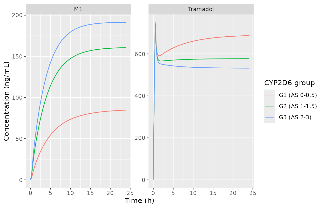
Typical-value tramadol and M1 profiles in a 3.2 kg, 40-week PMA neonate on the clinical intravenous regimen. Compare with the observed concentrations in Figure 3 of Healy 2025.
Figure 3 of the paper shows the observed concentrations as box plots by activity score, pooled over neonates of 31-54 weeks PMA sampled throughout the infusion, so this comparison is only qualitative. The observed tramadol medians are about 300-500 ng/mL; the typical-value prediction at 24 h (about 530-690 ng/mL) is at or above the upper end of that range. The observed median M1 concentrations are about 25-40 ng/mL at activity scores 0.5-1 and 70-100 ng/mL at 1.5-3. The typical-value M1 prediction (about 85-190 ng/mL) is roughly twice those medians; see “M1 exposure” under Assumptions and deviations.
Oral titration in children (Figure 4, Tables S1 and S2)
Virtual cohort
The paper sampled NHANES and CALIPER demographics into a virtual
population and stratified it into 5 kg weight bands, giving 100 patients
per scenario (PMA 51-976 weeks, 4.7-73.4 kg; Table 3). Those individual
records are not published. Here weight is drawn uniformly over the
published 4.7-73.4 kg range, which gives each weight band equal
representation. Age is read off CDC 50th-percentile weight-for-age
references (averaged across sexes) with lognormal scatter, and
postmenstrual age is 40 + 52.18 * age_years, clipped to the
published 51-976 weeks. The two genotype combinations the paper flags as
of clinical concern are simulated with 100 patients each, as in the
paper: CYP2D6 G3 with OCT1 G0, and CYP2D6 G2 with OCT1 G0.
rxode2::rxSetSeed(20250201)
set.seed(20250201)
n_per_arm <- 100L

# CDC 50th percentile weight for age, averaged across sexes.
growth <- tibble::tribble(
  ~age , ~wt  ,
  0.25 ,  6.0 ,
  0.50 ,  7.6 ,
  1.00 ,  9.6 ,
  2.00 , 12.2 ,
  3.00 , 14.3 ,
  4.00 , 16.3 ,
  5.00 , 18.3 ,
  6.00 , 20.6 ,
  7.00 , 23.0 ,
  8.00 , 25.6 ,
  10.00, 32.0 ,
  12.00, 40.5 ,
  14.00, 50.0 ,
  16.00, 58.0 ,
  18.00, 63.0
)

demog <- tibble::tibble(
  subj = seq_len(n_per_arm),
  WT = stats::runif(n_per_arm, 4.7, 73.4)
) |>
  dplyr::mutate(
    wt_ref = WT * exp(stats::rnorm(dplyr::n(), 0, 0.15)),
    age = stats::approx(growth$wt, growth$age, xout = wt_ref, rule = 2)$y,
    PAGE = pmin(pmax(40 + 52.18 * age, 51), 976),
    band = cut(
      WT,
      breaks = c(0, 10, 20, 40, Inf),
      right = FALSE,
      labels = c("<10", "10-<20", "20-<40", ">40")
    )
  ) |>
  dplyr::select(subj, WT, PAGE, band)

arms <- tibble::tibble(
  arm = c("CYP2D6-G3 + OCT1-G0", "CYP2D6-G2 + OCT1-G0"),
  CYP2D6_ASG2 = c(0, 1),
  CYP2D6_ASG3 = c(1, 0),
  OCT1_ASG1 = 0,
  OCT1_ASG2 = 0
)
cohort <- tidyr::crossing(arms, demog) |>
  dplyr::mutate(id = dplyr::row_number())

summary(demog[, c("WT", "PAGE")])
#>        WT              PAGE
#>  Min.   : 4.959   Min.   : 53.05
#>  1st Qu.:15.674   1st Qu.:267.00
#>  Median :35.721   Median :592.79
#>  Mean   :35.534   Mean   :546.51
#>  3rd Qu.:50.848   3rd Qu.:775.60
#>  Max.   :70.934   Max.   :976.00
Dosing and sampling
Table 4 titrates from 1 mg/kg/day on day 1 to 2, 3, 5 and 8 mg/kg/day on days 3, 5, 14 and 21. Doses are given orally three times daily, and the daily dose is capped at 400 mg. Figure 4 and Table S1 summarise one 24 h window at each step: day 2, day 4, day 13, day 20 and day 23 (24-48, 72-96, 288-312, 456-480 and 528-552 h).
steps <- tibble::tibble(
  step_start = c(0, 48, 96, 312, 480),
  step_end = c(48, 96, 312, 480, 552),
  mgkg = c(1, 2, 3, 5, 8)
)
windows <- tibble::tibble(
  start = c(24, 72, 288, 456, 528),
  end = c(48, 96, 312, 480, 552),
  dose = c(1, 2, 3, 5, 8),
  window = c(
    "Day 2 (1 mg/kg)",
    "Day 4 (2 mg/kg)",
    "Day 13 (3 mg/kg)",
    "Day 20 (5 mg/kg)",
    "Day 23 (8 mg/kg)"
  )
)

dose_times <- steps |>
  dplyr::rowwise() |>
  dplyr::reframe(
    time = seq(step_start, step_end - 8, by = 8),
    mgkg = mgkg
  )
doses <- tidyr::crossing(dplyr::select(cohort, id, WT), dose_times) |>
  dplyr::mutate(
    amt = pmin(mgkg * WT, 400) / 3,
    evid = 1L,
    cmt = "depot",
    dvid = NA_integer_
  ) |>
  dplyr::select(id, time, amt, evid, cmt, dvid)

obs_grid <- sort(unique(c(
  0,
  unlist(lapply(seq_len(nrow(windows)), function(i) {
    seq(windows$start[i], windows$end[i], by = 0.5)
  }))
)))
obs <- tidyr::crossing(id = cohort$id, time = obs_grid) |>
  dplyr::mutate(amt = NA_real_, evid = 0L, cmt = "central", dvid = 1L)

events <- dplyr::bind_rows(doses, obs) |>
  dplyr::left_join(
    dplyr::select(
      cohort,
      id,
      WT,
      PAGE,
      CYP2D6_ASG2,
      CYP2D6_ASG3,
      OCT1_ASG1,
      OCT1_ASG2
    ),
    by = "id"
  ) |>
  dplyr::arrange(id, time, dplyr::desc(evid)) |>
as.data.frame()Figure 4
target <- tibble::tibble(
  analyte = rep(c("Tramadol", "M1"), each = 2),
  conc = c(200, 300, 33, 50)
)
fig4 <- sim |>
  dplyr::filter(time > 0) |>
  dplyr::select(id, arm, time, Tramadol = Cc, M1 = Cc_m1) |>
  tidyr::pivot_longer(c(Tramadol, M1), names_to = "analyte", values_to = "conc") |>
  dplyr::inner_join(
    windows,
    by = dplyr::join_by(time >= start, time <= end)
  ) |>
  dplyr::group_by(arm, analyte, window, time) |>
  dplyr::summarise(
    med = stats::median(conc),
    lo = stats::quantile(conc, 0.025),
    hi = stats::quantile(conc, 0.975),
    .groups = "drop"
  ) |>
  dplyr::mutate(
    window = factor(window, levels = windows$window),
    analyte = factor(analyte, levels = c("Tramadol", "M1"))
  )
ggplot(fig4, aes(time, med)) +
  geom_ribbon(aes(ymin = lo, ymax = hi), fill = "grey80") +
  geom_line() +
  geom_hline(
    data = target,
    aes(yintercept = conc),
    linetype = "dashed",
    colour = "red"
  ) +
  facet_grid(arm + analyte ~ window, scales = "free") +
  labs(x = "Time (h)", y = "Concentration (ng/mL)") +
  theme(strip.text = element_text(size = 7))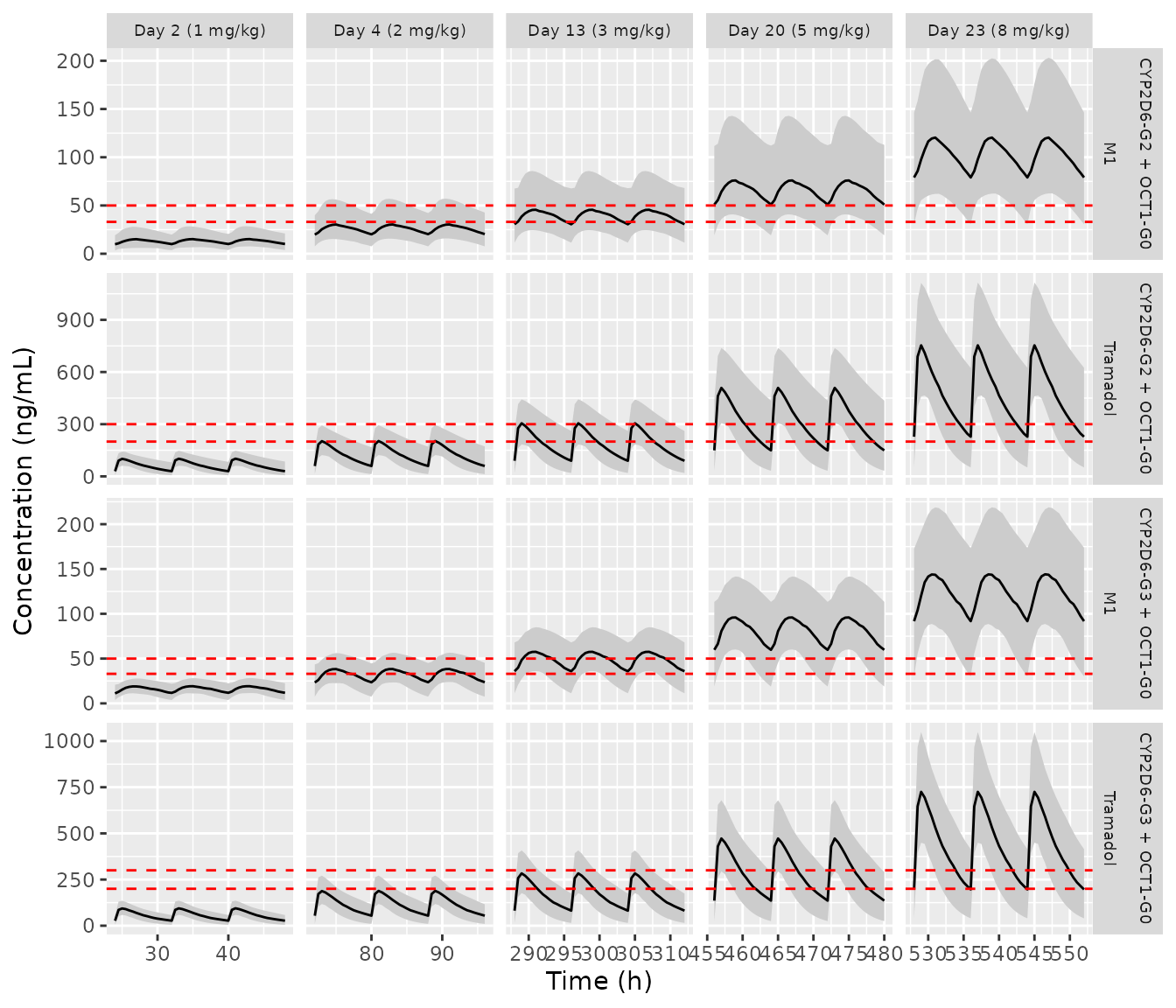
Replicates Figure 4 of Healy 2025: median (line) and 95% prediction interval (band) of tramadol and M1 concentrations in each titration window. Dashed lines mark the putative analgesic ranges (tramadol 200-300 ng/mL, M1 33-50 ng/mL).
PKNCA over each titration window
The paper’s AUC is the 24 h AUC of the window, and its Css is AUC /
24. This matches the Table S1 identity AUC = 24 * Css
(1335.63 = 24 x 55.65), so Css maps to PKNCA’s cav. Linear
trapezoids are used because the concentrations are close to steady
state.
nca_intervals <- windows |>
  dplyr::transmute(start, end, auclast = TRUE, cmax = TRUE, cav = TRUE)

run_nca <- function(conc_col) {
  conc_df <- sim |>
    dplyr::filter(!is.na(.data[[conc_col]])) |>
    dplyr::transmute(id, arm, time, conc = .data[[conc_col]])
  dose_df <- doses |>
    dplyr::left_join(dplyr::select(cohort, id, arm), by = "id") |>
    dplyr::select(id, arm, time, amt)
  conc_obj <- PKNCA::PKNCAconc(conc_df, conc ~ time | arm + id)
  dose_obj <- PKNCA::PKNCAdose(dose_df, amt ~ time | arm + id)
  dat <- PKNCA::PKNCAdata(
    conc_obj,
    dose_obj,
    intervals = nca_intervals,
    options = list(auc.method = "linear")
  )
  as.data.frame(PKNCA::pk.nca(dat)$result) |>
    dplyr::left_join(dplyr::select(windows, start, dose), by = "start")
}
nca_tram <- run_nca("Cc")
nca_m1 <- run_nca("Cc_m1")
Table S1 reports medians (90% prediction intervals). The reference values below are the medians.
ref_s1 <- function(arm_g3, arm_g2) {
  dplyr::bind_rows(
    dplyr::mutate(arm_g3, arm = "CYP2D6-G3 + OCT1-G0"),
    dplyr::mutate(arm_g2, arm = "CYP2D6-G2 + OCT1-G0")
  ) |>
    dplyr::mutate(dose = rep(c(1, 2, 3, 5, 8), 2)) |>
    dplyr::select(arm, dose, auclast, cav, cmax)
}
ref_tram <- ref_s1(
  tibble::tibble(
    auclast = c(1335.63, 2672.4, 4013.92, 6689.85, 9736.38),
    cav = c(55.65, 111.35, 167.25, 278.74, 405.68),
    cmax = c(82.01, 164.03, 246.07, 410.12, 597.72)
  ),
  tibble::tibble(
    auclast = c(1432.91, 2869.42, 4309.86, 7183.06, 10498.13),
    cav = c(59.7, 119.56, 179.58, 299.29, 437.42),
    cmax = c(85.71, 171.48, 257.29, 428.81, 628.25)
  )
)
ref_m1 <- ref_s1(
  tibble::tibble(
    auclast = c(169.98, 342.38, 517.21, 862.02, 1265.25),
    cav = c(7.08, 14.27, 21.55, 35.92, 52.72),
    cmax = c(8.05, 16.11, 24.18, 40.3, 61.67)
  ),
  tibble::tibble(
    auclast = c(138.28, 277.17, 419.05, 698.41, 1098.07),
    cav = c(5.76, 11.55, 17.46, 29.1, 45.75),
    cmax = c(6.65, 13.29, 19.94, 33.24, 51.79)
  )
)
nca_units <- c(auclast = "ng*h/mL", cav = "ng/mL", cmax = "ng/mL")
Tramadol (Table S1, upper panel)
cmp_tram <- nlmixr2lib::ncaComparisonTable(
  simulated = dplyr::select(nca_tram, arm, dose, PPTESTCD, PPORRES),
  reference = ref_tram,
  by = c("arm", "dose"),
  params = c("auclast", "cav", "cmax"),
  units = nca_units
)
knitr::kable(cmp_tram)| NCA parameter | arm | dose | Reference | Simulated | % diff |
|---|---|---|---|---|---|
| Cmax (ng/mL) | CYP2D6-G3 + OCT1-G0 | 1 | 82 | 95.3 | +16.2% |
| Cmax (ng/mL) | CYP2D6-G3 + OCT1-G0 | 2 | 164 | 191 | +16.3% |
| Cmax (ng/mL) | CYP2D6-G3 + OCT1-G0 | 3 | 246 | 287 | +16.4% |
| Cmax (ng/mL) | CYP2D6-G3 + OCT1-G0 | 5 | 410 | 478 | +16.4% |
| Cmax (ng/mL) | CYP2D6-G3 + OCT1-G0 | 8 | 598 | 725 | +21.3%* |
| Cmax (ng/mL) | CYP2D6-G2 + OCT1-G0 | 1 | 85.7 | 102 | +18.8% |
| Cmax (ng/mL) | CYP2D6-G2 + OCT1-G0 | 2 | 171 | 204 | +19.1% |
| Cmax (ng/mL) | CYP2D6-G2 + OCT1-G0 | 3 | 257 | 307 | +19.4% |
| Cmax (ng/mL) | CYP2D6-G2 + OCT1-G0 | 5 | 429 | 512 | +19.4% |
| Cmax (ng/mL) | CYP2D6-G2 + OCT1-G0 | 8 | 628 | 755 | +20.3%* |
| AUClast (ng*h/mL) | CYP2D6-G3 + OCT1-G0 | 1 | 1340 | 1380 | +3.2% |
| AUClast (ng*h/mL) | CYP2D6-G3 + OCT1-G0 | 2 | 2670 | 2760 | +3.2% |
| AUClast (ng*h/mL) | CYP2D6-G3 + OCT1-G0 | 3 | 4010 | 4140 | +3.1% |
| AUClast (ng*h/mL) | CYP2D6-G3 + OCT1-G0 | 5 | 6690 | 6900 | +3.1% |
| AUClast (ng*h/mL) | CYP2D6-G3 + OCT1-G0 | 8 | 9740 | 10500 | +7.5% |
| AUClast (ng*h/mL) | CYP2D6-G2 + OCT1-G0 | 1 | 1430 | 1510 | +5.6% |
| AUClast (ng*h/mL) | CYP2D6-G2 + OCT1-G0 | 2 | 2870 | 3050 | +6.2% |
| AUClast (ng*h/mL) | CYP2D6-G2 + OCT1-G0 | 3 | 4310 | 4600 | +6.6% |
| AUClast (ng*h/mL) | CYP2D6-G2 + OCT1-G0 | 5 | 7180 | 7660 | +6.6% |
| AUClast (ng*h/mL) | CYP2D6-G2 + OCT1-G0 | 8 | 10500 | 11400 | +8.4% |
| Cavg (ng/mL) | CYP2D6-G3 + OCT1-G0 | 1 | 55.6 | 57.4 | +3.2% |
| Cavg (ng/mL) | CYP2D6-G3 + OCT1-G0 | 2 | 111 | 115 | +3.2% |
| Cavg (ng/mL) | CYP2D6-G3 + OCT1-G0 | 3 | 167 | 172 | +3.1% |
| Cavg (ng/mL) | CYP2D6-G3 + OCT1-G0 | 5 | 279 | 287 | +3.1% |
| Cavg (ng/mL) | CYP2D6-G3 + OCT1-G0 | 8 | 406 | 436 | +7.5% |
| Cavg (ng/mL) | CYP2D6-G2 + OCT1-G0 | 1 | 59.7 | 63 | +5.6% |
| Cavg (ng/mL) | CYP2D6-G2 + OCT1-G0 | 2 | 120 | 127 | +6.2% |
| Cavg (ng/mL) | CYP2D6-G2 + OCT1-G0 | 3 | 180 | 191 | +6.6% |
| Cavg (ng/mL) | CYP2D6-G2 + OCT1-G0 | 5 | 299 | 319 | +6.6% |
| Cavg (ng/mL) | CYP2D6-G2 + OCT1-G0 | 8 | 437 | 474 | +8.4% |
M1 (Table S1, lower panel)
cmp_m1 <- nlmixr2lib::ncaComparisonTable(
  simulated = dplyr::select(nca_m1, arm, dose, PPTESTCD, PPORRES),
  reference = ref_m1,
  by = c("arm", "dose"),
  params = c("auclast", "cav", "cmax"),
  units = nca_units
)
knitr::kable(cmp_m1)| NCA parameter | arm | dose | Reference | Simulated | % diff |
|---|---|---|---|---|---|
| Cmax (ng/mL) | CYP2D6-G3 + OCT1-G0 | 1 | 8.05 | 19.3 | +139.6%* |
| Cmax (ng/mL) | CYP2D6-G3 + OCT1-G0 | 2 | 16.1 | 38.6 | +139.4%* |
| Cmax (ng/mL) | CYP2D6-G3 + OCT1-G0 | 3 | 24.2 | 57.9 | +139.3%* |
| Cmax (ng/mL) | CYP2D6-G3 + OCT1-G0 | 5 | 40.3 | 96.4 | +139.3%* |
| Cmax (ng/mL) | CYP2D6-G3 + OCT1-G0 | 8 | 61.7 | 145 | +135.5%* |
| Cmax (ng/mL) | CYP2D6-G2 + OCT1-G0 | 1 | 6.65 | 15.2 | +128.8%* |
| Cmax (ng/mL) | CYP2D6-G2 + OCT1-G0 | 2 | 13.3 | 30.5 | +129.2%* |
| Cmax (ng/mL) | CYP2D6-G2 + OCT1-G0 | 3 | 19.9 | 45.8 | +129.7%* |
| Cmax (ng/mL) | CYP2D6-G2 + OCT1-G0 | 5 | 33.2 | 76.3 | +129.7%* |
| Cmax (ng/mL) | CYP2D6-G2 + OCT1-G0 | 8 | 51.8 | 121 | +132.9%* |
| AUClast (ng*h/mL) | CYP2D6-G3 + OCT1-G0 | 1 | 170 | 382 | +124.5%* |
| AUClast (ng*h/mL) | CYP2D6-G3 + OCT1-G0 | 2 | 342 | 774 | +126.0%* |
| AUClast (ng*h/mL) | CYP2D6-G3 + OCT1-G0 | 3 | 517 | 1160 | +124.9%* |
| AUClast (ng*h/mL) | CYP2D6-G3 + OCT1-G0 | 5 | 862 | 1940 | +124.9%* |
| AUClast (ng*h/mL) | CYP2D6-G3 + OCT1-G0 | 8 | 1270 | 2910 | +129.6%* |
| AUClast (ng*h/mL) | CYP2D6-G2 + OCT1-G0 | 1 | 138 | 308 | +122.4%* |
| AUClast (ng*h/mL) | CYP2D6-G2 + OCT1-G0 | 2 | 277 | 618 | +122.9%* |
| AUClast (ng*h/mL) | CYP2D6-G2 + OCT1-G0 | 3 | 419 | 944 | +125.4%* |
| AUClast (ng*h/mL) | CYP2D6-G2 + OCT1-G0 | 5 | 698 | 1570 | +125.4%* |
| AUClast (ng*h/mL) | CYP2D6-G2 + OCT1-G0 | 8 | 1100 | 2430 | +121.3%* |
| Cavg (ng/mL) | CYP2D6-G3 + OCT1-G0 | 1 | 7.08 | 15.9 | +124.5%* |
| Cavg (ng/mL) | CYP2D6-G3 + OCT1-G0 | 2 | 14.3 | 32.2 | +125.9%* |
| Cavg (ng/mL) | CYP2D6-G3 + OCT1-G0 | 3 | 21.6 | 48.5 | +124.9%* |
| Cavg (ng/mL) | CYP2D6-G3 + OCT1-G0 | 5 | 35.9 | 80.8 | +124.9%* |
| Cavg (ng/mL) | CYP2D6-G3 + OCT1-G0 | 8 | 52.7 | 121 | +129.6%* |
| Cavg (ng/mL) | CYP2D6-G2 + OCT1-G0 | 1 | 5.76 | 12.8 | +122.4%* |
| Cavg (ng/mL) | CYP2D6-G2 + OCT1-G0 | 2 | 11.6 | 25.7 | +122.8%* |
| Cavg (ng/mL) | CYP2D6-G2 + OCT1-G0 | 3 | 17.5 | 39.4 | +125.4%* |
| Cavg (ng/mL) | CYP2D6-G2 + OCT1-G0 | 5 | 29.1 | 65.6 | +125.4%* |
| Cavg (ng/mL) | CYP2D6-G2 + OCT1-G0 | 8 | 45.8 | 101 | +121.3%* |
Tramadol by weight band (Table S2)
Table S2 stratifies the same scenarios by weight band, which separates the genotype effect from growth and maturation. It depends much less on the assumed weight distribution than the pooled Table S1. The tramadol Css medians at 1 and 5 mg/kg/day are compared below. The M1 block of Table S2 is printed with its rows shifted between weight bands and doses, so it is not used.
ref_s2 <- tibble::tribble(
  ~arm                  , ~dose , ~band    , ~cav  ,
  "CYP2D6-G3 + OCT1-G0" ,     1 , "<10"    ,  37.3 ,
  "CYP2D6-G3 + OCT1-G0" ,     1 , "10-<20" ,  45.3 ,
  "CYP2D6-G3 + OCT1-G0" ,     1 , "20-<40" ,  52.3 ,
  "CYP2D6-G3 + OCT1-G0" ,     1 , ">40"    ,  62.4 ,
  "CYP2D6-G3 + OCT1-G0" ,     5 , "<10"    , 186.7 ,
  "CYP2D6-G3 + OCT1-G0" ,     5 , "10-<20" , 226.6 ,
  "CYP2D6-G3 + OCT1-G0" ,     5 , "20-<40" , 262.2 ,
  "CYP2D6-G3 + OCT1-G0" ,     5 , ">40"    , 313.7 ,
  "CYP2D6-G2 + OCT1-G0" ,     1 , "<10"    ,  41.4 ,
  "CYP2D6-G2 + OCT1-G0" ,     1 , "10-<20" ,  48.8 ,
  "CYP2D6-G2 + OCT1-G0" ,     1 , "20-<40" ,  57.2 ,
  "CYP2D6-G2 + OCT1-G0" ,     1 , ">40"    ,  67.5 ,
  "CYP2D6-G2 + OCT1-G0" ,     5 , "<10"    , 207.0 ,
  "CYP2D6-G2 + OCT1-G0" ,     5 , "10-<20" , 244.9 ,
  "CYP2D6-G2 + OCT1-G0" ,     5 , "20-<40" , 286.5 ,
  "CYP2D6-G2 + OCT1-G0" ,     5 , ">40"    , 339.5
)
sim_s2 <- nca_tram |>
  dplyr::filter(PPTESTCD == "cav", dose %in% c(1, 5)) |>
  dplyr::left_join(dplyr::distinct(cohort, id, band), by = "id") |>
  dplyr::mutate(band = as.character(band)) |>
  dplyr::select(arm, dose, band, PPTESTCD, PPORRES)
cmp_s2 <- nlmixr2lib::ncaComparisonTable(
  simulated = sim_s2,
  reference = ref_s2,
  by = c("arm", "dose", "band"),
  params = "cav",
  units = nca_units
)
knitr::kable(cmp_s2)| NCA parameter | arm | dose | band | Reference | Simulated | % diff |
|---|---|---|---|---|---|---|
| Cavg (ng/mL) | CYP2D6-G3 + OCT1-G0 | 1 | <10 | 37.3 | 42.7 | +14.5% |
| Cavg (ng/mL) | CYP2D6-G3 + OCT1-G0 | 1 | 10-<20 | 45.3 | 47.8 | +5.5% |
| Cavg (ng/mL) | CYP2D6-G3 + OCT1-G0 | 1 | 20-<40 | 52.3 | 48.7 | -6.8% |
| Cavg (ng/mL) | CYP2D6-G3 + OCT1-G0 | 1 | >40 | 62.4 | 70.1 | +12.3% |
| Cavg (ng/mL) | CYP2D6-G3 + OCT1-G0 | 5 | <10 | 187 | 214 | +14.5% |
| Cavg (ng/mL) | CYP2D6-G3 + OCT1-G0 | 5 | 10-<20 | 227 | 239 | +5.5% |
| Cavg (ng/mL) | CYP2D6-G3 + OCT1-G0 | 5 | 20-<40 | 262 | 244 | -7.1% |
| Cavg (ng/mL) | CYP2D6-G3 + OCT1-G0 | 5 | >40 | 314 | 354 | +12.8% |
| Cavg (ng/mL) | CYP2D6-G2 + OCT1-G0 | 1 | <10 | 41.4 | 45.5 | +9.8% |
| Cavg (ng/mL) | CYP2D6-G2 + OCT1-G0 | 1 | 10-<20 | 48.8 | 52.8 | +8.2% |
| Cavg (ng/mL) | CYP2D6-G2 + OCT1-G0 | 1 | 20-<40 | 57.2 | 61.9 | +8.2% |
| Cavg (ng/mL) | CYP2D6-G2 + OCT1-G0 | 1 | >40 | 67.5 | 70.8 | +4.9% |
| Cavg (ng/mL) | CYP2D6-G2 + OCT1-G0 | 5 | <10 | 207 | 228 | +10.0% |
| Cavg (ng/mL) | CYP2D6-G2 + OCT1-G0 | 5 | 10-<20 | 245 | 265 | +8.0% |
| Cavg (ng/mL) | CYP2D6-G2 + OCT1-G0 | 5 | 20-<40 | 286 | 310 | +8.0% |
| Cavg (ng/mL) | CYP2D6-G2 + OCT1-G0 | 5 | >40 | 340 | 355 | +4.6% |
Checks
pct <- function(tbl) {
  as.numeric(gsub("[%*+]", "", tbl[["% diff"]]))
}
s2_diff <- pct(cmp_s2)
s1_tram_diff <- pct(cmp_tram[cmp_tram[["NCA parameter"]] != "Cmax (ng/mL)", ])

# M1 at steady state: d(central_m1) = d(peripheral1_m1) = 0 gives
# Cc_m1 / Cc = CLPM / (0.947 * CLMO), whatever VM1, VM2 or QM are. On day 23
# the 8 mg/kg/day step has run for 48 h, so the window average is close to
# steady state for nearly every subject. A subject who draws a very large VM1
# with a slow M1 elimination is still approaching it, so the check uses the
# centre and a robust quantile rather than every subject.
ind <- sim |>
  dplyr::filter(time == 552) |>
  dplyr::distinct(id, cl_form_m1, cl_m1)
ratio_chk <- nca_m1 |>
  dplyr::filter(PPTESTCD == "cav", dose == 8) |>
  dplyr::select(id, cav_m1 = PPORRES) |>
  dplyr::inner_join(
    nca_tram |>
      dplyr::filter(PPTESTCD == "cav", dose == 8) |>
      dplyr::select(id, cav_tram = PPORRES),
    by = "id"
  ) |>
  dplyr::inner_join(ind, by = "id") |>
  dplyr::mutate(
    pct_diff = 100 *
      (cav_m1 / cav_tram / (cl_form_m1 / (0.947 * cl_m1)) - 1)
  )

stopifnot(
  # Tramadol by weight band: the cohort-robust comparison. A mis-transcribed
  # clearance, maturation or allometric term moves these by tens of percent.
  abs(stats::median(s2_diff)) < 15,
  stats::quantile(abs(s2_diff), 0.9) < 25,
  # Tramadol AUC and Cavg pooled over the cohort (Table S1); this depends on
  # the assumed weight distribution as well as the model.
  abs(stats::median(s1_tram_diff)) < 15,
  # M1 steady-state identity: both sides use the same drawn parameters.
  abs(stats::median(ratio_chk$pct_diff)) < 2,
  stats::quantile(abs(ratio_chk$pct_diff), 0.9) < 5
)
Assumptions and deviations
-
M1 exposure. Simulated M1 concentrations are about
2.2-fold above the medians the paper reports in Table S1 for both
genotype combinations, while tramadol agrees closely, especially by
weight band (Table S2). At steady state the M1/tramadol concentration
ratio of this model is
CLPM / (0.947 * CLMO)(checked per subject above). It does not depend on VM1, VM2, QM or their random effects, and CLMO has no random effect in the final control stream. For CYP2D6 G3 with OCT1 G0 the ratio is 14.7 / (0.947 x 57.7) = 0.27, whereas Tables S1 and S2 imply about 0.12-0.13. The paper’s 90% prediction intervals for M1 (for example 0.88-45.55 ng/mL at 1 mg/kg/day) span about 50-fold, far wider than the control-stream model can produce. That width is consistent with an M1-clearance random effect of variance about 1.45 (the VM1 variance, whoseETA(7)index the commented-outCLMO = TVCLMO;*EXP(ETA(7))line also uses). The paper’s simulation code therefore probably differs from the published control stream in the M1 arm, but neither the code nor any other reported value reconciles the medians. The model is packaged exactly as Table 5 and the control stream specify, and no value has been adjusted to match the simulated M1 tables. The neonatal check above points the same way: the typical-value M1 prediction lies above the medians observed in Figure 3. - Tramadol Cmax. Simulated tramadol AUC and Cavg agree with Table S1 within about 8%, but the simulated median Cmax is 16-21% higher. Cmax depends on ka and VP1, which do not affect AUC. The paper reports no variability on ka and no other absorption detail, so the difference is reported here rather than resolved.
-
Residual error mapping. Table 5 labels the four
residual variances “proportional tramadol 0.0159, additive tramadol
0.01, proportional M1 0.00001, additive M1 0.00004”. The executed
control stream assigns
$SIGMA0.0159 FIX and 0.00001 FIX toEPS(1)andEPS(2), the tramadol proportional and additive terms in$ERROR. The two estimatedEPS(3)andEPS(4)are the M1 proportional and additive terms. The$SIGMAcomments (CVCP,CVCM) suggest the authors read the second fixed value as the M1 proportional error, so the table labels follow that reading rather than the code. The model follows the code: tramadol proportional SD sqrt(0.0159), additive SD sqrt(0.00001) ng/mL (both fixed), M1 proportional SD sqrt(0.01) and additive SD sqrt(0.00004) ng/mL. Under either reading the additive terms are negligible. The code reading also gives a plausible 10% M1 proportional error instead of 0.3%. Residual error does not enter any simulation in this article. -
Vestigial CLPP thetas. The control stream assigns
CLPP = THETA(1-3)(28.7 / 36.3 / 43, fixed, from the tramadol-only step) by CYP2D6 group, then overwrites it withCLPP = CLPO + CLPM. CLPP never enters$DES, so those three values are not model parameters. The model exposescl_total = cl + cl_form_m1as a derived output. -
Molar ratio. The 0.947 factor multiplies only the
two outflows from the M1 central compartment, exactly as in
$DES. The observation isA3 / VM1without the factor. - Oral bioavailability. The model was fitted to intravenous data. Ka (1.28 1/h) comes from an external capsule study, and no bioavailability is reported, so F = 1 is implicit. Tramadol agreement with Tables S1 and S2 is consistent with the paper’s simulations also using F = 1.
-
Fixed-status. QP, VP1 and VP2 were estimated in the
tramadol-only step (Table 5 lists their RSEs) and are
FIXin the final joint control stream, so they are encoded withfixed(). The same applies to the$SIGMAvalues 0.0159 and 0.00001. - Virtual cohort. Individual NHANES/CALIPER records are not published. Weight is drawn uniformly over 4.7-73.4 kg (the paper stratified by 5 kg weight band), and age comes from CDC weight-for-age references. This cohort has a lower median weight than the 45 kg in Table 3. The weight-band comparison against Table S2 does not depend on this choice. The Table S1 comparison does, which is why its check is looser.
- Dosing schedule. Doses are given every 8 h from time 0, with each step starting at the beginning of its Table 4 day. The 400 mg/day cap is applied per daily dose.