Gentamicin (Bijleveld 2017)

Model and source

• Citation: Bijleveld YA, van den Heuvel ME, Hodiamont CJ, Mathot RAA, de Haan TR. Population pharmacokinetics and dosing considerations for gentamicin in newborns with suspected or proven sepsis caused by gram-negative bacteria. Antimicrob Agents Chemother. 2017;61(1):e01304-16.
• Article: https://doi.org/10.1128/AAC.01304-16

mod_meta <- rxode2::rxode(readModelDb("Bijleveld_2017_gentamicin"))
#> ℹ parameter labels from comments will be replaced by 'label()'
mod_meta$description
#> [1] "Two-compartment population PK model of intravenous gentamicin in (pre)term neonates with suspected or proven Gram-negative sepsis (Bijleveld 2017), with fixed allometric body-weight scaling (exponents 0.75 on CL and Q, 1 on Vc and Vp) and an estimated postmenstrual-age power effect on CL."
mod_meta$reference
#> [1] "Bijleveld YA, van den Heuvel ME, Hodiamont CJ, Mathot RAA, de Haan TR. Population pharmacokinetics and dosing considerations for gentamicin in newborns with suspected or proven sepsis caused by gram-negative bacteria. Antimicrob Agents Chemother. 2017;61(1):e01304-16. doi:10.1128/AAC.01304-16."
mod_meta$units
#> $time
#> [1] "hour"
#> 
#> $dosing
#> [1] "mg"
#> 
#> $concentration
#> [1] "mg/L"

Population

Bijleveld 2017 developed an allometric two-compartment population PK model from 65 (pre)term neonates treated with intravenous gentamicin in the NICU of the Academic Medical Center, Amsterdam, between October 2012 and January 2013 (Bijleveld 2017 Table 1). Demographics: 37 male and 28 female, mean gestational age 32 weeks (range 25-42), with 75% of the cohort born prematurely (GA < 37 weeks). Body weight at the start of treatment had a median of 1.85 kg (range 0.76-4.67 kg) and birth weight had the same median value (range 0.43-4.67 kg). Postnatal age at the start of treatment had a median of 1 day (range 0-31). Serum creatinine averaged 55.5 umol/L (range 26-112), and mortality during the observation window was 8%. A total of 136 gentamicin serum concentrations (median 2 per subject, range 1-4) were available for the final PK analysis. Doses were 4 mg/kg every 48 h (GA <= 32 wk, PNA < 4 wk), 4 mg/kg every 24 h (GA > 32 wk, PNA < 4 wk), or 5 mg/kg every 24 h (PNA > 4 wk), administered as 30-min IV infusions.

The same information is available programmatically via readModelDb("Bijleveld_2017_gentamicin")$population.

Source trace

The per-parameter origin is recorded as an in-file comment next to each ini() entry in inst/modeldb/specificDrugs/Bijleveld_2017_gentamicin.R. The table below collects them in one place for review.

Equation / parameter	Value	Source location
lcl (log CL per 70 kg)	log(1.00)	Bijleveld 2017 Table 3, Final Model column
lvc (log Vc per 70 kg)	log(37.4)	Bijleveld 2017 Table 3, Final Model column
lq (log Q per 70 kg)	log(0.57)	Bijleveld 2017 Table 3, Final Model column
lvp (log Vp per 70 kg)	log(17.1)	Bijleveld 2017 Table 3, Final Model column
e_wt_cl_q (allometric exp on CL, Q)	0.75 (fixed)	Bijleveld 2017 Table 3 footnotes b, d
e_wt_vc_vp (allometric exp on Vc, Vp)	1 (fixed)	Bijleveld 2017 Table 3 footnotes c, e
e_page_cl (PMA/225 d power on CL)	1.89 (theta_ClPMA)	Bijleveld 2017 Table 3, Final Model column
IIV CL (omega^2 = log(1 + 0.331^2))	0.10396 (33.1% CV)	Bijleveld 2017 Table 3, IIV CL
IIV Vc (omega^2 = log(1 + 0.244^2))	0.05784 (24.4% CV)	Bijleveld 2017 Table 3, IIV Vc
Cor(IIV CL, IIV Vc) -> covariance	0.08 * sqrt(0.10396 * 0.05784) = 0.006204	Bijleveld 2017 Results, “Pharmacokinetic model” paragraph
expSd (lognormal residual SD)	0.43	Bijleveld 2017 Table 3, Additive error (residual variability of log-transformed data)
Two-compartment IV PK ODE structure	n/a	Bijleveld 2017 Results, “Pharmacokinetic model” (allometric 2-compartment)
Log-additive (LTBS) -> lnorm residual	n/a	Bijleveld 2017 Results, “Pharmacokinetic model”; residual variability described on log-transformed data
Reference body weight 70 kg	n/a	Bijleveld 2017 Table 3 footnotes (CL liters/h/70 kg, Vc liters/70 kg)
Reference PMA 225 days	n/a	Bijleveld 2017 Table 3 footnote b (median PMA = 32 wk + 1 d ~= 225 d)

Virtual cohort

The original observed data are not publicly available. The vignette draws four virtual cohorts to mirror the Bijleveld 2017 Monte Carlo scenarios (Table 4 and Figure 4): each cohort fixes one of the gestational-age / body-weight pairs the paper tabulated and applies the recommended 5 mg/kg per-dose regimen for that GA stratum. Postmenstrual age is supplied at every observation row so it advances correctly over the 7-day simulation window (the paper computes PMA as the sum of GA days and PNA days, and CL scales with PMA via the power exponent 1.89).

The paper used 1,000 patients per arm; the vignette uses 300 to stay inside the pkgdown build time budget while keeping Monte Carlo noise below ~3 percentage points on each target-attainment statistic. The canonical covariate names in the model are WT (kg) and PAGE (postmenstrual age in months); the cohort table below applies the required day-to-month conversion (PAGE = PMA_days / 30.4375).

set.seed(20260602)

n_subjects <- 300L
infusion_h <- 0.5     # 30 min infusion (Bijleveld 2017 Methods)
duration_h <- 7 * 24  # 7-day simulation window per Methods "Pharmacokinetic analysis and simulations"

# Bijleveld 2017 Table 4 / Figure 4 anchor scenarios. PNA is set to
# 0 days at the start of treatment to match the paper's Monte Carlo
# initialisation (PMA = GA + PNA).
regimens <- tibble::tribble(
  ~regimen,           ~ga_weeks, ~wt_kg, ~dose_mg_per_kg, ~interval_h,
  "GA 25 wk q48h",    25,        0.830,  5,               48,
  "GA 32 wk q36h",    32,        2.000,  5,               36,
  "GA 37 wk q24h",    37,        2.500,  5,               24,
  "GA 40 wk q24h",    40,        3.500,  5,               24
)

obs_grid <- sort(unique(c(
  seq(0, 2, by = 0.1),                       # peri-peak resolution
  seq(2, duration_h, by = 1)                 # hourly through 7 days
)))

make_cohort <- function(n, regimen, ga_weeks, wt_kg, dose_mg_per_kg,
                        interval_h, id_offset = 0L) {
  ids       <- id_offset + seq_len(n)
  ga_days   <- ga_weeks * 7
  amt_mg    <- wt_kg * dose_mg_per_kg
  dose_times <- seq(0, duration_h - 1, by = interval_h)

  dose_rows <- tidyr::expand_grid(id = ids, time = dose_times) |>
    dplyr::mutate(
      evid = 1L,
      cmt  = "central",
      amt  = amt_mg,
      rate = amt_mg / infusion_h,
      WT   = wt_kg,
      # PMA advances with simulation time: PMA_days = GA_days + t/24 (PNA = 0 at t=0)
      PAGE    = (ga_days + time / 24) / 30.4375,
      regimen = regimen
    )

  obs_rows <- tidyr::expand_grid(id = ids, time = obs_grid) |>
    dplyr::mutate(
      evid = 0L,
      cmt  = "central",
      amt  = 0,
      rate = 0,
      WT   = wt_kg,
      PAGE    = (ga_days + time / 24) / 30.4375,
      regimen = regimen
    )

  dplyr::bind_rows(dose_rows, obs_rows) |>
    dplyr::arrange(id, time, dplyr::desc(evid))
}

events <- dplyr::bind_rows(
  make_cohort(n_subjects, regimens$regimen[1], regimens$ga_weeks[1],
              regimens$wt_kg[1], regimens$dose_mg_per_kg[1],
              regimens$interval_h[1], id_offset =    0L),
  make_cohort(n_subjects, regimens$regimen[2], regimens$ga_weeks[2],
              regimens$wt_kg[2], regimens$dose_mg_per_kg[2],
              regimens$interval_h[2], id_offset = 1000L),
  make_cohort(n_subjects, regimens$regimen[3], regimens$ga_weeks[3],
              regimens$wt_kg[3], regimens$dose_mg_per_kg[3],
              regimens$interval_h[3], id_offset = 2000L),
  make_cohort(n_subjects, regimens$regimen[4], regimens$ga_weeks[4],
              regimens$wt_kg[4], regimens$dose_mg_per_kg[4],
              regimens$interval_h[4], id_offset = 3000L)
)

stopifnot(!anyDuplicated(unique(events[, c("id", "time", "evid")])))

cat(
  "Dose rows:", sum(events$evid == 1L),
  " | Obs rows:", sum(events$evid == 0L), "\n"
)
#> Dose rows: 6900  | Obs rows: 224400

Simulation

mod <- readModelDb("Bijleveld_2017_gentamicin")
sim <- rxode2::rxSolve(
  mod,
  events = events,
  keep   = c("regimen", "WT", "PAGE")
) |>
  as.data.frame()
#> ℹ parameter labels from comments will be replaced by 'label()'

Replicate published figures

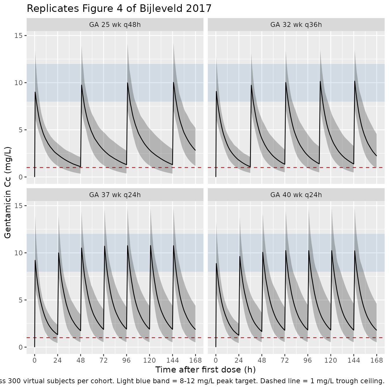
Figure 4 – concentration-time profiles for recommended regimens

Bijleveld 2017 Figure 4 shows the median and 5th-95th percentile concentration-time profiles for the recommended dosing regimens by GA stratum: 5 mg/kg every 48 h for GA < 37 wk, every 36 h for GA 37-40 wk, and every 24 h for GA >= 40 wk. The shaded region covers the target peak range of 8-12 mg/L and the horizontal line at 1 mg/L marks the maximum acceptable trough. The chunk below renders the same panel across the four anchor cohorts in the virtual population.

ribbon_df <- sim |>
  dplyr::filter(!is.na(Cc)) |>
  dplyr::group_by(regimen, time) |>
  dplyr::summarise(
    Q05 = quantile(Cc, 0.05, na.rm = TRUE),
    Q50 = quantile(Cc, 0.50, na.rm = TRUE),
    Q95 = quantile(Cc, 0.95, na.rm = TRUE),
    .groups = "drop"
  )

ggplot(ribbon_df, aes(time, Q50)) +
  annotate("rect", xmin = -Inf, xmax = Inf, ymin = 8, ymax = 12,
           alpha = 0.15, fill = "steelblue") +
  geom_hline(yintercept = 1, linetype = "dashed", colour = "firebrick") +
  geom_ribbon(aes(ymin = Q05, ymax = Q95), alpha = 0.30) +
  geom_line() +
  facet_wrap(~regimen, ncol = 2) +
  scale_x_continuous(breaks = seq(0, 168, 24)) +
  labs(
    x       = "Time after first dose (h)",
    y       = "Gentamicin Cc (mg/L)",
    title   = "Replicates Figure 4 of Bijleveld 2017",
    caption = paste0(
      "Median (solid) and 5th-95th percentile (shaded) gentamicin profiles ",
      "across ", n_subjects, " virtual subjects per cohort. ",
      "Light blue band = 8-12 mg/L peak target. ",
      "Dashed line = 1 mg/L trough ceiling."
    )
  )

PKNCA validation

Compute Cmax (peak) and Cmin (trough) per subject over the final dosing interval using PKNCA, grouped by regimen. The paper defines peak as the concentration 30 minutes after the end of a 30-minute infusion, i.e. one hour after dose start; trough is the concentration immediately before the next dose. The PKNCA cmax over the closed interval matches this definition because the simulated peak occurs at the end of the infusion.

# Take the steady-state interval after dose 4 (or, for q24h, dose 7).
# We use the last full dosing interval before the simulation ends.
last_dose_start <- sapply(regimens$interval_h, function(int) {
  # most recent dose start such that start + interval <= duration
  starts <- seq(0, duration_h - 1, by = int)
  max(starts[starts + int <= duration_h])
})
names(last_dose_start) <- regimens$regimen
last_dose_end <- last_dose_start + regimens$interval_h
names(last_dose_end) <- regimens$regimen

sim_nca <- sim |>
  dplyr::filter(!is.na(Cc)) |>
  dplyr::group_by(regimen) |>
  dplyr::mutate(
    interval_start = last_dose_start[as.character(regimen)],
    interval_end   = last_dose_end[as.character(regimen)]
  ) |>
  dplyr::filter(time >= interval_start, time <= interval_end) |>
  dplyr::mutate(time_in_interval = time - interval_start) |>
  dplyr::ungroup() |>
  dplyr::select(id, time_in_interval, Cc, regimen)

conc_obj <- PKNCA::PKNCAconc(
  sim_nca, Cc ~ time_in_interval | regimen + id,
  concu = "mg/L", timeu = "h"
)

# Dose at t = 0 of the last interval; amount per cohort
dose_amt <- regimens$wt_kg * regimens$dose_mg_per_kg
names(dose_amt) <- regimens$regimen

dose_df <- sim_nca |>
  dplyr::distinct(id, regimen) |>
  dplyr::mutate(
    time_in_interval = 0,
    amt              = dose_amt[as.character(regimen)]
  )

dose_obj <- PKNCA::PKNCAdose(
  dose_df, amt ~ time_in_interval | regimen + id,
  doseu = "mg"
)

intervals <- data.frame(
  start    = 0,
  end      = max(regimens$interval_h),
  cmax     = TRUE,
  cmin     = TRUE,
  tmax     = TRUE,
  auclast  = TRUE
)

nca_data <- PKNCA::PKNCAdata(conc_obj, dose_obj, intervals = intervals)
nca_res  <- PKNCA::pk.nca(nca_data)
res_tbl  <- as.data.frame(nca_res$result)

Comparison against Bijleveld 2017 Table 4

Bijleveld 2017 Table 4 reports simulated median trough and peak concentrations (with IQR) for each GA / regimen combination. The chunk below recomputes those statistics from the simulated subject-level peaks (taken at t = 1 hour into the last dosing interval, matching the paper’s Cmax definition) and troughs (taken at the end of the last interval) and renders them side-by-side with the published values.

peak_h <- 1.0   # 30 min after the end of a 30 min infusion

simulated <- sim |>
  dplyr::group_by(regimen) |>
  dplyr::mutate(
    interval_start = last_dose_start[as.character(regimen)],
    interval_end   = last_dose_end[as.character(regimen)]
  ) |>
  dplyr::ungroup()

peaks <- simulated |>
  dplyr::filter(abs((time - interval_start) - peak_h) < 1e-6) |>
  dplyr::select(id, regimen, peak = Cc)

troughs <- simulated |>
  dplyr::group_by(id, regimen) |>
  dplyr::filter(time >= interval_start, time <= interval_end) |>
  dplyr::slice_max(time, n = 1, with_ties = FALSE) |>
  dplyr::ungroup() |>
  dplyr::select(id, regimen, trough = Cc)

simulated_summary <- dplyr::left_join(peaks, troughs, by = c("id", "regimen")) |>
  dplyr::group_by(regimen) |>
  dplyr::summarise(
    median_trough_sim = median(trough, na.rm = TRUE),
    median_peak_sim   = median(peak,   na.rm = TRUE),
    iqr_trough_sim    = paste0(
      sprintf("%.2f-%.2f",
              quantile(trough, 0.25, na.rm = TRUE),
              quantile(trough, 0.75, na.rm = TRUE))
    ),
    iqr_peak_sim      = paste0(
      sprintf("%.2f-%.2f",
              quantile(peak, 0.25, na.rm = TRUE),
              quantile(peak, 0.75, na.rm = TRUE))
    ),
    .groups = "drop"
  )

published <- tibble::tribble(
  ~regimen,         ~median_trough_pub, ~iqr_trough_pub, ~median_peak_pub, ~iqr_peak_pub,
  "GA 25 wk q48h",  1.26,               "0.82-1.83",     9.72,             "8.41-11.18",
  "GA 32 wk q36h",  1.34,               "0.86-1.96",     9.81,             "8.48-11.33",
  "GA 37 wk q24h",  1.82,               "1.21-2.66",     10.29,            "8.87-11.82",
  "GA 40 wk q24h",  1.61,               "1.05-2.39",     10.08,            "8.71-11.57"
)

comparison <- published |>
  dplyr::left_join(simulated_summary, by = "regimen") |>
  dplyr::select(regimen,
                median_trough_pub, median_trough_sim, iqr_trough_pub, iqr_trough_sim,
                median_peak_pub,   median_peak_sim,   iqr_peak_pub,   iqr_peak_sim)

knitr::kable(
  comparison,
  digits  = 2,
  caption = paste("Comparison of simulated trough and peak concentrations with",
                  "Bijleveld 2017 Table 4 (5 mg/kg regimens). The 'pub' columns",
                  "are the published median (with interquartile range, mg/L);",
                  "the 'sim' columns are recomputed from the packaged model.")
)

Comparison of simulated trough and peak concentrations with Bijleveld 2017 Table 4 (5 mg/kg regimens). The ‘pub’ columns are the published median (with interquartile range, mg/L); the ‘sim’ columns are recomputed from the packaged model.

regimen	median_trough_pub	median_trough_sim	iqr_trough_pub	iqr_trough_sim	median_peak_pub	median_peak_sim	iqr_peak_pub	iqr_peak_sim
GA 25 wk q48h	1.26	1.31	0.82-1.83	0.90-2.07	9.72	9.98	8.41-11.18	8.87-11.68
GA 32 wk q36h	1.34	1.38	0.86-1.96	0.91-2.16	9.81	10.14	8.48-11.33	8.98-11.69
GA 37 wk q24h	1.82	1.86	1.21-2.66	1.25-2.70	10.29	10.76	8.87-11.82	9.47-12.29
GA 40 wk q24h	1.61	1.78	1.05-2.39	1.09-2.62	10.08	10.22	8.71-11.57	9.00-11.67

The simulated medians should track the published Table 4 values within Monte Carlo noise (1,000 vs 300 subjects per arm). The single covariate effect on CL is the postmenstrual-age power exponent of 1.89, so the GA-to-GA gradient in steady-state exposure is driven almost entirely by that term and by the linear allometric scaling of all four PK parameters with body weight.

knitr::kable(
  res_tbl[, c("start", "end", "regimen", "PPTESTCD", "PPORRES")],
  caption = "Per-subject PKNCA NCA parameters by regimen (long form, first 24 rows shown).",
  digits  = 3,
  row.names = FALSE
) |>
  utils::head()
#> [1] "Table: Per-subject PKNCA NCA parameters by regimen (long form, first 24 rows shown)."
#> [2] ""                                                                                    
#> [3] "| start| end|regimen       |PPTESTCD | PPORRES|"                                     
#> [4] "|-----:|---:|:-------------|:--------|-------:|"                                     
#> [5] "|     0|  48|GA 25 wk q48h |auclast  | 125.978|"                                     
#> [6] "|     0|  48|GA 25 wk q48h |cmax     |   8.352|"

Assumptions and deviations

• Postmenstrual age set time-varying from PNA = 0. Bijleveld 2017’s Methods and Monte Carlo description compute PMA as the sum of GA and PNA in days; the vignette initialises each virtual subject at PNA = 0 on the first dose and lets PMA advance with simulation time. The source paper’s Table 4 simulations were “for a 7-day period”, which matches this 168-hour window. Median PMA in the source cohort was 225 days, consistent with mean GA 32 weeks plus median PNA 1 day.
• Body weight held constant per cohort over 7 days. The paper applies allometric scaling to body weight at the start of treatment; the simulated 7-day window is short enough that weight gain is not expected to materially change the CL or volume terms. Users running longer windows or modelling neonates with rapid weight gain should encode WT as a time-varying covariate.
• PNA, gender, and ibuprofen co-medication not in the final model. The paper tested these covariates and reported no significant improvement over the PMA-only model; the packaged model carries only the PMA effect on CL.
• Residual error encoded as lognormal (lnorm(expSd)) with sigma = 0.43. The paper describes the residual variability on log-transformed observations as additive with sigma = 0.43. The log-additive NONMEM pattern (log(Cobs) = log(Cpred) + eps, eps ~ N(0, sigma^2)) maps directly to nlmixr2’s lnorm() residual with expSd = sigma. For small sigma this also approximates a proportional residual with propSd = sigma, but at sigma = 0.43 the approximation is no longer exact (~4% difference in implied CV), so the lognormal form is preferred.
• Infusion duration set by the event table. The model does not hard-code dur(central). Users specify infusion duration per dose via the rate (or dur) column on event-table dose rows; the vignette uses rate = amt / 0.5 to deliver each dose over 30 minutes.
• Cmax definition. The paper’s peak is the concentration 30 minutes after the end of a 30-minute infusion (i.e. one hour after the start of a dose). The comparison table uses that definition; the PKNCA cmax over the closed interval matches because the simulated peak always occurs at the end of infusion in the absence of post-infusion rebound from distribution.
• Allometric exponents fixed. Bijleveld 2017 Table 3 footnotes report the body-weight exponents as 0.75 (CL, Q) and 1 (Vc, Vp) without uncertainty; these are wrapped in fixed() in the packaged model. The PMA exponent on CL (theta_ClPMA = 1.89) is reported with CV 26%, indicating it was estimated rather than fixed, and is left free in the packaged model.
• Errata not located. A targeted search of the journal landing page and Google Scholar at extraction time did not turn up an erratum for this article. If one is later identified that revises a Table 3 estimate, the packaged values should be refreshed accordingly.