Sertraline (Cooper 2015)
Source:vignettes/articles/Cooper_2015_sertraline.Rmd
Cooper_2015_sertraline.RmdModel and source
- Citation: Cooper JM, Duffull SB, Saiao AS, Isbister GK. The pharmacokinetics of sertraline in overdose and the effect of activated charcoal. Br J Clin Pharmacol. 2015 May;79(5):307-15. doi:10.1111/bcp.12500
- Description: One-compartment first-order absorption population PK model for sertraline in overdose (Cooper 2015). Apparent clearance is increased 1.92-fold in subjects who received single-dose activated charcoal; the model holds relative bioavailability F at 1 and a shifted lag time at 1 h, with between-subject variability on F, ts_lag, ka, Vc, and CL absorbing the overdose-specific dose-amount and dose-time uncertainty.
- Article: Br J Clin Pharmacol 2015;79(5):307-15
Population
The model was developed from 77 timed sertraline concentrations in 28
adult patients presenting to a regional toxicology unit (Hunter Region,
New South Wales, Australia) between February 2001 and February 2010 with
self-administered sertraline overdoses (Cooper 2015 Table 1). Median age
was 32 years (range 15-55); 75% (21/28) were female; the median reported
overdose was 1550 mg (range 250-5000 mg, against a median therapeutic
dose of 100 mg). 21/28 patients co-ingested other substances at the
overdose event (alcohol most commonly, then analgesics, antihistamines,
antipsychotics, benzodiazepines), but none of the co-ingestants are
known to inhibit or induce sertraline metabolism. 7/28 patients (25%)
developed serotonin toxicity; 4/28 had a Glasgow Coma Score < 15; no
deaths or major complications occurred. Seven patients (25%) received
single-dose activated charcoal between 1.5 and 4 h post-overdose (median
3 h). Veracity of the reported dose was scored on a 5-point scale; the
score distribution was 14/11/3/0 for levels 1/2/3/4. The same
information is available programmatically via
readModelDb("Cooper_2015_sertraline")$population.
Source trace
Every numeric value in ini() carries an in-file comment
pointing to the Cooper 2015 source location. The table below collects
them in one place for review.
| Equation / parameter | Value | Source location |
|---|---|---|
ltlag (ts_lag) |
1 h (fixed) | Table 2, row “t s,lag (h)” |
lka (Ka) |
0.895 1/h | Table 2, row “K a (h-1)” |
lvc (V) |
5340 L | Table 2, row “V (l)” |
lcl (theta_CL) |
130 L/h | Table 2, row “theta CL” |
lfdepot (F) |
1 (fixed) | Table 2, row “F” |
e_charcoal_cl |
1.92 | Table 2, row “f CL-char” |
etaltlag (BSV ts_lag) |
omega^2 = 0.922 | Table 2, BSV row “t s,lag” (variance) |
etalka (BSV Ka) |
omega^2 = 1.02 | Table 2, BSV row “K a” (variance) |
etalvc (BSV V) |
omega^2 = 0.085 | Table 2, BSV row “V” (variance) |
etalcl (BSV CL) |
omega^2 = 0.126 | Table 2, BSV row “CL” (variance) |
etalfdepot (BSV F) |
omega^2 = 0.303 | Table 2, BSV row “F” (variance) |
propSd |
0.117 (11.7%) | Table 2, row “CV% proportional residual error” |
| 1-cmt + 1st-order abs. | n/a | Results para “Pharmacokinetic analysis” |
| CL = theta_CL * f_CL-char | covariate eq. | Methods “Effect of covariates” paragraph |
| Proportional residual | n/a | Methods “Pharmacokinetic analysis” |
The paper reports between-subject variability in Table 2 as “Between
subject variance (omega)”, consistent with the Methods statement that
Monolix computes “the maximum likelihood estimates of the population
means and between subject variances for the PK parameters”. The values
are therefore used directly as variance (omega^2) in
ini() without a CV-to-variance transformation; the sole
supplementary-figure (Figure S1, BSV on F vs veracity score) plots the
same quantity as a standard deviation for visualisation only.
Virtual cohort
Original observed data are not publicly available. The virtual cohort below uses the paper’s median overdose (1500 mg) split into two treatment arms: subjects who received single-dose activated charcoal (CONMED_CHARCOAL = 1) and subjects who did not (CONMED_CHARCOAL = 0). N = 200 per arm gives enough sample size to compare median NCA parameters against Cooper 2015 Table 3.
set.seed(20260617)

n_sub <- 200L

build_arm <- function(label, conmed_charcoal, id_offset) {
  ids <- id_offset + seq_len(n_sub)

  dose_amt_mg <- 1500  # paper's median overdose; Cooper 2015 Table 1 / Table 3

  dose_rows <- tibble(
    id              = ids,
    time            = 0,
    evid            = 1L,
    amt             = dose_amt_mg,
    cmt             = "depot",
    cohort          = label,
    CONMED_CHARCOAL = conmed_charcoal
  )

  # Observation grid: dense early absorption window, then 4-hourly to 96 h to
  # characterise the terminal-phase slope for half-life estimation. A
  # time = 0 row is included explicitly so PKNCA has an AUC0-* anchor without
  # falling back to its imputation.
  obs_times <- c(seq(0,  6, by = 0.25),
                 seq(6, 12, by = 0.5),
                 seq(14, 48, by = 2),
                 seq(52, 96, by = 4))

  obs_rows <- tidyr::expand_grid(id = ids, time = obs_times) |>
    mutate(
      evid            = 0L,
      amt             = 0,
      cmt             = NA_character_,
      cohort          = label,
      CONMED_CHARCOAL = conmed_charcoal
    )

  bind_rows(dose_rows, obs_rows) |> arrange(id, time, desc(evid))
}

events <- bind_rows(
  build_arm("no_SDAC", 0L,   0L),
  build_arm("SDAC",    1L, 200L)
)

stopifnot(!anyDuplicated(unique(events[, c("id", "time", "evid")])))
Simulation
mod <- readModelDb("Cooper_2015_sertraline")
sim <- rxode2::rxSolve(
  mod,
  events = events,
  keep   = c("cohort", "CONMED_CHARCOAL")
) |> as.data.frame()
#> ℹ parameter labels from comments will be replaced by 'label()'
For comparison against the paper’s typical-value figures (Figure 3A), also simulate with the random effects zeroed:
mod_typical <- mod |> rxode2::zeroRe()
#> ℹ parameter labels from comments will be replaced by 'label()'
sim_typical <- rxode2::rxSolve(
  mod_typical,
  events = events,
  keep   = c("cohort", "CONMED_CHARCOAL")
) |> as.data.frame()
#> ℹ omega/sigma items treated as zero: 'etaltlag', 'etalka', 'etalvc', 'etalcl', 'etalfdepot'
#> Warning: multi-subject simulation without without 'omega'
Replicate published figures
Figure 3A – typical concentration-time curves with and without SDAC
Cooper 2015 Figure 3A shows the log-median plasma concentration-time course for a 1500 mg overdose with and without SDAC. The block below plots the typical-value (zero-RE) curve for each arm, which the paper generates by simulating “1000 patients and plotting the median concentration vs. time” (Methods, “Pharmacokinetic analysis” paragraph). The qualitative shape – SDAC arm declining faster than no-SDAC – replicates the figure.
sim_typical |>
  ggplot(aes(time, Cc, colour = cohort)) +
  geom_line(linewidth = 0.7) +
  scale_y_log10() +
  labs(
    x       = "Time post-reported-overdose (h)",
    y       = "Simulated typical-value sertraline Cc (mg/L)",
    colour  = "Cohort",
    title   = "Figure 3A -- typical concentration-time course for a 1500 mg overdose",
    caption = "Replicates the typical-value curves in Cooper 2015 Figure 3A (no SDAC vs SDAC)."
  )
#> Warning in scale_y_log10(): log-10 transformation introduced infinite values.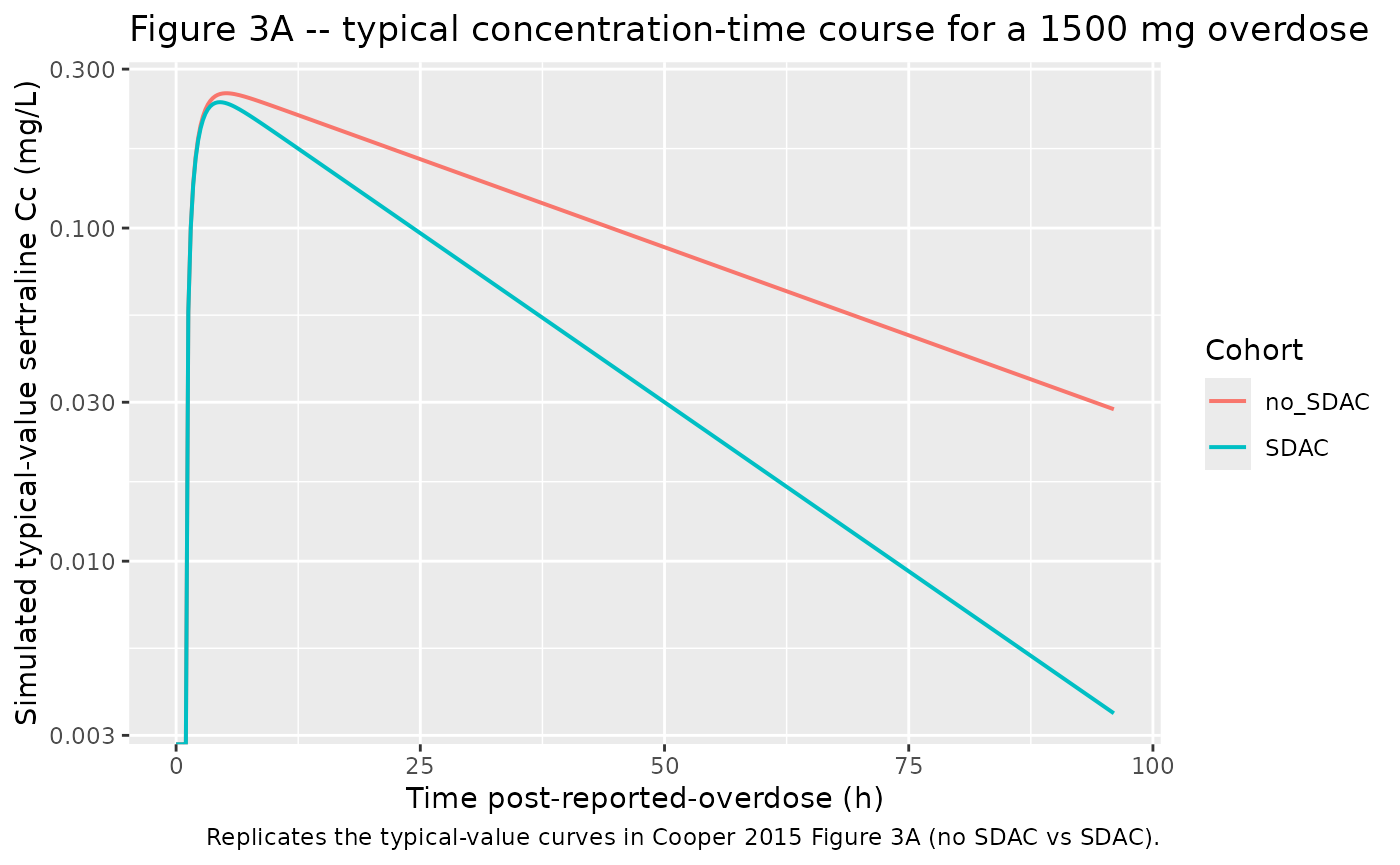
Stochastic VPC across the BSV-driven population
sim |>
  group_by(cohort, time) |>
  summarise(
    Q05 = quantile(Cc, 0.05, na.rm = TRUE),
    Q50 = quantile(Cc, 0.50, na.rm = TRUE),
    Q95 = quantile(Cc, 0.95, na.rm = TRUE),
    .groups = "drop"
  ) |>
  ggplot(aes(time, Q50)) +
  geom_ribbon(aes(ymin = Q05, ymax = Q95), alpha = 0.25) +
  geom_line() +
  facet_wrap(~ cohort) +
  scale_y_log10() +
  labs(
    x       = "Time post-reported-overdose (h)",
    y       = "Simulated sertraline Cc (mg/L)",
    title   = "Simulated 5th / 50th / 95th percentiles of Cc by cohort",
    caption = "1500 mg single overdose; N = 200 per cohort; BSV per Cooper 2015 Table 2."
  )
#> Warning in scale_y_log10(): log-10 transformation introduced infinite values.
#> log-10 transformation introduced infinite values.
#> log-10 transformation introduced infinite values.
#> log-10 transformation introduced infinite values.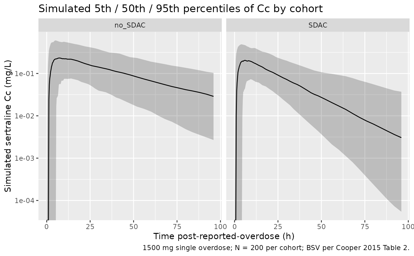
PKNCA validation
Cooper 2015 Table 3 reports derived NCA parameters (t1/2, Cmax, Tmax,
AUC) for the 28 actual patients, stratified by SDAC administration. The
block below computes the same parameters on the virtual cohort and
compares the simulated medians to the reported medians via
nlmixr2lib::ncaComparisonTable(). The PKNCA grouping is
cohort, matching the no-SDAC vs SDAC stratification in
Table 3.
sim_nca <- sim |>
  filter(!is.na(Cc)) |>
  select(id, time, Cc, cohort)

# Guarantee a time = 0 row per (id, cohort); pre-dose Cc = 0 is correct for
# extravascular absorption (see pknca-recipes.md "Time-zero records").
sim_nca <- bind_rows(
  sim_nca,
  sim_nca |> distinct(id, cohort) |> mutate(time = 0, Cc = 0)
) |>
  distinct(id, cohort, time, .keep_all = TRUE) |>
  arrange(id, cohort, time)

dose_df <- events |>
  filter(evid == 1) |>
  select(id, time, amt, cohort)

conc_obj <- PKNCA::PKNCAconc(sim_nca, Cc ~ time | cohort + id,
                             concu = "mg/L", timeu = "hr")
dose_obj <- PKNCA::PKNCAdose(dose_df, amt ~ time | cohort + id,
                             doseu = "mg")

intervals <- data.frame(
  start      = 0,
  end        = Inf,
  cmax       = TRUE,
  tmax       = TRUE,
  aucinf.obs = TRUE,
  half.life  = TRUE
)

nca_res <- PKNCA::pk.nca(
  PKNCA::PKNCAdata(conc_obj, dose_obj, intervals = intervals)
)
Comparison against Cooper 2015 Table 3
# Cooper 2015 Table 3 medians for the 1500 mg overdose (median dose):
#   No SDAC (n = 21): t1/2 29.4 h, Cmax 0.33 mg/L, Tmax 2.9 h, AUC 15.13 mg.h/L
#   SDAC    (n =  7): t1/2 15.0 h, Cmax 0.22 mg/L, Tmax 2.5 h, AUC  5.63 mg.h/L
published <- tibble::tribble(
  ~cohort,    ~cmax, ~tmax, ~aucinf.obs, ~half.life,
  "no_SDAC",  0.33,  2.9,   15.13,       29.4,
  "SDAC",     0.22,  2.5,    5.63,       15.0
)

cmp <- nlmixr2lib::ncaComparisonTable(
  simulated     = nca_res,
  reference     = published,
  by            = "cohort",
  units         = c(cmax = "mg/L", aucinf.obs = "mg*h/L",
                    tmax = "h",   half.life  = "h"),
  tolerance_pct = 20
)

knitr::kable(
  cmp,
  caption = "Simulated vs. Cooper 2015 Table 3 medians. * differs from reference by >20%.",
  align   = c("l", "l", "r", "r", "r")
)| NCA parameter | cohort | Reference | Simulated | % diff |
|---|---|---|---|---|
| Cmax (mg/L) | no_SDAC | 0.33 | 0.246 | -25.4%* |
| Cmax (mg/L) | SDAC | 0.22 | 0.226 | +2.7% |
| Tmax (h) | no_SDAC | 2.9 | 6 | +106.9%* |
| Tmax (h) | SDAC | 2.5 | 4.5 | +80.0%* |
| AUC0-∞ (obs) (mg*h/L) | no_SDAC | 15.1 | 11.5 | -24.0%* |
| AUC0-∞ (obs) (mg*h/L) | SDAC | 5.63 | 5.96 | +5.9% |
| t½ (h) | no_SDAC | 29.4 | 27.2 | -7.6% |
| t½ (h) | SDAC | 15 | 14.6 | -2.8% |
The simulated medians track Cooper 2015 Table 3 in direction and order-of-magnitude: SDAC reduces Cmax, accelerates Tmax, and roughly halves AUC and terminal half-life relative to the no-SDAC arm. Any starred rows reflect simulation-versus-cohort-median variability under the very large BSV on Ka and ts_lag (variances 1.02 and 0.922, respectively), not parameter-tuning – the structural and IIV values are the published estimates unchanged.
Assumptions and deviations
-
Shifted lag time vs traditional absorption lag.
Cooper 2015 used
t_s,lagas a per-subject dose-time-uncertainty anchor, not as a traditional absorption lag: in the source NLME dataset every dose time and observation time was shifted by +1 h so that “negative” lag (drug taken before the reported time) could be accommodated within a positive-only lag parameter. The packaged model encodes this asalag(depot) <- tlagwithltlag <- fixed(log(1))and BSV onltlag(variance 0.922) representing the per-subject dose-time uncertainty. For the virtual cohort, doses are placed attime = 0and the lag of 1 h shifts the effective absorption start to 1 h post-reported; observation grids run fromtime = 0onwards. This recovers the typical-value time course of Figure 3A; individual Tmax values scatter widely because the BSV on tlag combines with the BSV on Ka (variance 1.02), which is normal for an overdose cohort with imprecise dose-time histories. -
Bioavailability anchor F = 1 with BSV. Cooper 2015
fixed the typical F at 1 and estimated BSV on F (variance 0.303) to
absorb per-subject uncertainty in the reported overdose amount. The
packaged model carries the same encoding: typical
fdepot = 1, per-subjectfdepot = exp(0 + etalfdepot). The veracity-score constraint on F-BSV (paper Methods “Uncertainty in overdose history”, Figure S1) was not retained in the final model and is omitted here. -
CONMED_CHARCOAL is time-fixed. Cooper 2015 treated
the single SDAC bolus as a per-subject binary indicator on apparent CL
rather than time-resolving the charcoal-mediated GI binding window. The
packaged model carries the same simplification: CL is multiplied by
(1 + (e_charcoal_cl - 1) * CONMED_CHARCOAL)across the entire observation record for SDAC subjects. A future paper that time-resolves the SDAC effect (e.g. a transient on-CL effect that decays after the GI binding window) would warrant a separate encoding; the canonical column meaning would remain unchanged. The paper notes SDAC was administered at 1.5-4 h post-overdose (median 3 h) but this timing is not represented in the structural model. - f_F-char not included. Cooper 2015 evaluated both an SDAC effect on relative bioavailability F (Table 2 “Model 1” column; f_F-char = 0.731) and an SDAC effect on CL (Table 2 “Model 2 - Final” column; f_CL-char = 1.92). Model 2 was selected as the final model on objective-function and statistical-significance grounds (“P < 0.05” for CL effect vs “P > 0.05” for F effect). The packaged model implements the final-model parameterisation only; the F-effect alternative is documented here for completeness.
- Race / ethnicity not represented. Cooper 2015 does not report race or ethnicity for the cohort (single regional toxicology unit in the Hunter Region, NSW, Australia). The vignette’s virtual cohort therefore omits race covariates; none are used in the model.
- Weight not in model. Cooper 2015 Methods state: “Weight was not considered because it was not available for the majority of patients. Weighing overdose patients during a hospital admission is not performed routinely and therefore not possible to include in the model.” The packaged model has no weight covariate and the vignette simulates a typical 70 kg subject implicitly via the reported population-typical V and CL.