Imipenem in critically ill adults, parametric vs nonparametric (de Velde 2020)
Source:vignettes/articles/deVelde_2020_imipenem.Rmd
deVelde_2020_imipenem.RmdModel and source
de Velde 2020 fitted two population PK models to the same imipenem dataset from critically ill adults: a parametric model in NONMEM 7.2 (FOCE-I) and a nonparametric model in Pmetrics 1.5.2 (NPAG). The two were built independently to a pre-specified workflow and converged on the same structure: two compartments, parameterised in micro-constants, with absolute (BSA-unadjusted) CKD-EPI eGFR as a power covariate on the elimination rate constant. Both are packaged here.
mod_par <- readModelDb("deVelde_2020_imipenem")
mod_np <- readModelDb("deVelde_2020_imipenem_nonparametric")- Parametric (NONMEM): Two-compartment IV population PK model for imipenem in 26 critically ill adults treated with imipenem-cilastatin in a Geneva intensive care unit (de Velde 2020, parametric NONMEM arm), parameterised in micro-constants rather than clearances: an elimination rate constant, two distribution rate constants and a central volume. The elimination rate constant scales as a power of absolute (BSA-unadjusted) CKD-EPI eGFR in mL/min, entered as a time-varying covariate. Between-subject variability is exponential on the elimination rate constant only, and residual error is additive on log-transformed concentrations. The same data were also fitted non-parametrically in Pmetrics; that arm is the sibling model deVelde_2020_imipenem_nonparametric.
- Nonparametric (Pmetrics NPAG): Two-compartment IV population PK model for imipenem in 26 critically ill adults treated with imipenem-cilastatin in a Geneva intensive care unit (de Velde 2020, non-parametric Pmetrics NPAG arm), parameterised in micro-constants: an elimination rate constant, two distribution rate constants and a central volume. The elimination rate constant scales as a power of absolute (BSA-unadjusted) CKD-EPI eGFR in mL/min. NPAG places every parameter, including the covariate exponent, in a discrete joint density; that density is approximated here by independent log-normal marginals matched to the published mean and CV%. Residual error is the Pmetrics gamma-scaled assay polynomial, a linear sum of additive and proportional terms. The parametric NONMEM arm fitted to the same data is the sibling model deVelde_2020_imipenem.
- Citation: de Velde F, de Winter BCM, Neely MN, Yamada WM, Koch BCP, Harbarth S, von Dach E, van Gelder T, Huttner A, Mouton JW, on behalf of COMBACTE-NET consortium. Population pharmacokinetics of imipenem in critically ill patients: a parametric and nonparametric model converge on CKD-EPI estimated glomerular filtration rate as an impactful covariate. Clin Pharmacokinet. 2020;59(7):885-898. doi:10.1007/s40262-020-00859-1
- Article (open access): https://doi.org/10.1007/s40262-020-00859-1
deVelde_2020_imipenem was first added to this package
from the Zhang 2025 imipenem systematic review (see the Zhang 2025 review
article). It has since been re-verified against this primary
publication, and the nonparametric arm was added at the same time. The
differences the primary exposed are listed under “Assumptions and
deviations” below.
Population
Data came from a prospective cohort study (2010-2013) in the intensive care unit of the Geneva University Hospitals, Switzerland. Of 54 imipenem-treated patients, the last 27 had exact dosing and sampling times recorded; one was excluded for missing height, leaving 26. Inclusion required suspected or documented severe bacterial infection and age 18-60 years; exclusion criteria were Cockcroft-Gault eGFR below 60 mL/min, BMI below 18 or above 30 kg/m^2, and pregnancy. The cohort was 69% male, median age 51 years (IQR 39-54), median weight 75 kg (IQR 66-85), median BSA 1.89 m^2, and median APACHE II score 22. Renal function was high: median CKD-EPI 116 mL/min/1.73 m^2 and CKD-EPI-abs 119 mL/min at inclusion. Most infections were lower respiratory tract (62%). No patient received continuous renal replacement therapy (Table 1, Sect. 2.1, Sect. 3.1).
Patients received imipenem/cilastatin 500 mg/500 mg four times daily as a 30-min intravenous infusion. 138 plasma samples (peak, intermediate and trough on days 1, 2, 3, 4 and 6) were assayed by HPLC-UV; the 13 below the 0.5 mg/L limit of quantification were excluded, leaving 125 concentrations after 84 doses (Sect. 3.2).
str(mod_par()$population[c("n_subjects", "n_concentrations", "regions", "renal_function")])
#> List of 4
#>  $ n_subjects      : int 26
#>  $ n_concentrations: int 125
#>  $ regions         : chr "Switzerland (Geneva University Hospitals ICU)"
#>  $ renal_function  : chr "CKD-EPI 116 mL/min/1.73 m^2 (IQR 104-124); CKD-EPI-abs 119 mL/min (IQR 110-139); Cockcroft-Gault 146 mL/min (IQ"| __truncated__
Source trace
The per-parameter origin is also recorded as an in-file comment next
to each ini() entry in both model files.
| Equation / parameter | NONMEM model | Pmetrics model | Source location |
|---|---|---|---|
| Two-compartment structure, micro-constants | yes | yes | Sect. 3.3 / 3.4 (1-cmt dOFV +22.99 / d-2LL +26.5; 3-cmt no gain) |
lkel (Ke at CRCL = 119) |
log(0.637) | log(0.681) | Table 2 |
lk12 (Kcp) |
log(0.166) | log(0.374) | Table 2 |
lk21 (Kpc) |
log(0.195) | log(0.495) | Table 2 |
lvc (Vc) |
log(29.6) | log(31.1) | Table 2 |
e_crcl_kel (Ke(cov)) |
0.655 | 0.658 | Table 2; Eq. 9 / Eq. 10 |
kel = Ke x (CRCL/119)^Ke(cov) x e^eta |
yes | yes (exponent also random) | Eq. 9 / Eq. 10; 119 = median CKD-EPI-abs (Table 1) |
etalkel |
0.0354 | log(0.340^2 + 1) | Sect. 3.3 (omega^2 = 0.0354); Table 2 CV 34.0% |
etalk12, etalk21, etalvc
|
none | log(CV^2 + 1) from 81.2%, 72.0%, 42.6% | Sect. 3.3 (no BSV on Vc, Kcp, Kpc); Table 2 |
etae_crcl_kel |
none | log(0.552^2 + 1) | Table 2 (Ke(cov) CV 55.2%) |
| Residual error |
lnorm(expSd), expSd = 0.348 |
add(0.17) + prop(0.17) + combined1() |
Eq. 1 and Table 2; Eqs. 3 and 5, gamma 3.40 (Table 2), C0 = C1 = 0.05 (Sect. 3.4) |
d/dt(central), d/dt(peripheral1)
|
yes | yes | standard two-compartment micro-constant ODEs |
The Pmetrics residual error follows from Eqs. 3 and 5,
error = gamma x (C0 + C1 x OBS), so the SD is
3.40 x 0.05 + 3.40 x 0.05 x C = 0.17 + 0.17 x C mg/L.
Closed-form checks against the published parameters
Neither model is fitted here, so the first validation is that the packaged files reproduce the paper’s own derived quantities exactly.
omega_cv <- function(mod, eta) {
  om <- rxode2::rxode(mod)$omega
  sqrt(exp(om[eta, eta]) - 1)
}
typical <- function(mod) {
  th <- rxode2::rxode(mod)$theta
  kel <- exp(th[["lkel"]]); k12 <- exp(th[["lk12"]]); k21 <- exp(th[["lk21"]])
  vc  <- exp(th[["lvc"]])
  a <- kel + k12 + k21
  beta <- (a - sqrt(a^2 - 4 * k21 * kel)) / 2
  alpha <- k21 * kel / beta
  c(kel = kel, vc = vc, cl = kel * vc, vss = vc * (1 + k12 / k21),
    thalf_alpha = log(2) / alpha, thalf_beta = log(2) / beta)
}
tv <- rbind(NONMEM = typical(mod_par), Pmetrics = typical(mod_np))
#> ℹ parameter labels from comments will be replaced by 'label()'
#> ℹ parameter labels from comments will be replaced by 'label()'

checks <- tibble::tribble(
  ~Check, ~Published, ~Model,
  "NONMEM Ke CV (Table 2, Eq. 2)", 0.190, omega_cv(mod_par, "etalkel"),
  "NONMEM Ke SD, 1/h (Fig. 1)", 0.121, 0.637 * omega_cv(mod_par, "etalkel"),
  "Pmetrics Ke CV (Table 2)", 0.340, omega_cv(mod_np, "etalkel"),
  "Pmetrics Kcp CV (Table 2)", 0.812, omega_cv(mod_np, "etalk12"),
  "Pmetrics Kpc CV (Table 2)", 0.720, omega_cv(mod_np, "etalk21"),
  "Pmetrics Vc CV (Table 2)", 0.426, omega_cv(mod_np, "etalvc"),
  "Pmetrics Ke(cov) CV (Table 2)", 0.552, omega_cv(mod_np, "etae_crcl_kel")
) |>
  mutate(`Rel. diff` = signif(Model / Published - 1, 2), Model = signif(Model, 4))
#> ℹ parameter labels from comments will be replaced by 'label()'
#> ℹ parameter labels from comments will be replaced by 'label()'
#> ℹ parameter labels from comments will be replaced by 'label()'
#> ℹ parameter labels from comments will be replaced by 'label()'
#> ℹ parameter labels from comments will be replaced by 'label()'
#> ℹ parameter labels from comments will be replaced by 'label()'
#> ℹ parameter labels from comments will be replaced by 'label()'
knitr::kable(checks, caption = "Between-subject variability reproduced from the packaged omegas.")| Check | Published | Model | Rel. diff |
|---|---|---|---|
| NONMEM Ke CV (Table 2, Eq. 2) | 0.190 | 0.1898 | -9.1e-04 |
| NONMEM Ke SD, 1/h (Fig. 1) | 0.121 | 0.1209 | -6.7e-04 |
| Pmetrics Ke CV (Table 2) | 0.340 | 0.3400 | -1.8e-06 |
| Pmetrics Kcp CV (Table 2) | 0.812 | 0.8120 | -4.0e-07 |
| Pmetrics Kpc CV (Table 2) | 0.720 | 0.7200 | -2.0e-07 |
| Pmetrics Vc CV (Table 2) | 0.426 | 0.4260 | 1.6e-06 |
| Pmetrics Ke(cov) CV (Table 2) | 0.552 | 0.5520 | -4.0e-07 |
# Identities of the encoded omegas: the only slack is the paper's rounding.
stopifnot(all(abs(checks$`Rel. diff`) < 0.006))

knitr::kable(signif(tv, 4), caption = paste(
  "Typical-subject (CRCL = 119 mL/min) derived quantities. CL = Vc x Ke is",
  "the clearance quoted in the Discussion."
))| kel | vc | cl | vss | thalf_alpha | thalf_beta | |
|---|---|---|---|---|---|---|
| NONMEM | 0.637 | 29.6 | 18.86 | 54.8 | 0.8133 | 4.756 |
| Pmetrics | 0.681 | 31.1 | 21.18 | 54.6 | 0.5380 | 2.649 |
The typical NONMEM clearance, Vc x Ke = 18.9 L/h, is the
value the Discussion calls higher than earlier imipenem models in
critically ill patients and attributes to augmented renal clearance.
Imipenem’s disposition is dominated by the alpha phase (half-life 0.81 h
in the NONMEM model), consistent with the roughly 1 h half-life the
Introduction quotes for normal renal function.
Virtual cohort and simulation
The paper’s Electronic Supplementary Fig. 4 simulates each model at CKD-EPI-abs 150, 120 and 90 mL/min. The same three renal-function levels are used here, with 200 virtual patients per model and level, on the study regimen of 500 mg every 6 h as a 30-min infusion for 4 days. CKD-EPI-abs is held constant per patient (the source analysis treated it as time-varying; see “Assumptions and deviations”).
set.seed(2020)
rxode2::rxSetSeed(2020)

n_per_arm <- 200L
crcl_levels <- c(150, 120, 90)
dose_times <- seq(0, 90, by = 6)
obs_times <- sort(unique(c(seq(90, 96, by = 0.25), 90.5)))

make_cohort <- function(crcl, id_offset) {
  ids <- id_offset + seq_len(n_per_arm)
  dose <- expand.grid(id = ids, time = dose_times) |>
    mutate(evid = 1L, amt = 500, rate = 1000, cmt = "central")
  obs <- expand.grid(id = ids, time = obs_times) |>
    mutate(evid = 0L, amt = 0, rate = 0, cmt = "central")
  bind_rows(dose, obs) |>
    mutate(CRCL = crcl, egfr = paste0("CKD-EPI-abs ", crcl, " mL/min")) |>
    arrange(id, time, desc(evid))
}
events <- bind_rows(lapply(seq_along(crcl_levels), function(i) {
  make_cohort(crcl_levels[i], id_offset = (i - 1L) * n_per_arm)
}))
stopifnot(!anyDuplicated(unique(events[, c("id", "time", "evid")])))
sim_one <- function(mod, label) {
  rxode2::rxSolve(mod, events = events, keep = c("egfr", "CRCL"),
                  returnType = "data.frame") |>
    mutate(model = label)
}
sim <- bind_rows(
  sim_one(mod_par, "NONMEM (parametric)"),
  sim_one(mod_np, "Pmetrics (nonparametric)")
) |>
  mutate(tad = time - 90,
         egfr = factor(egfr, levels = paste0("CKD-EPI-abs ", crcl_levels, " mL/min")))
#> ℹ parameter labels from comments will be replaced by 'label()'
#> ℹ parameter labels from comments will be replaced by 'label()'
Replicate published figures
# Replicates Electronic Supplementary Fig. 4 of de Velde 2020: simulated
# concentration-time profiles by CKD-EPI-abs for each model. `Cc` is the
# individual prediction (no residual error).
band <- sim |>
  group_by(model, egfr, tad) |>
  summarise(
    P025 = quantile(Cc, 0.025), P50 = median(Cc), P975 = quantile(Cc, 0.975),
    .groups = "drop"
  )
ggplot(band, aes(tad, P50, colour = model, fill = model)) +
  geom_ribbon(aes(ymin = P025, ymax = P975), alpha = 0.2, colour = NA) +
  geom_line() +
  facet_wrap(~egfr, ncol = 1) +
  scale_y_log10() +
  labs(x = "Time after dose (h), steady state", y = "Imipenem (mg/L)",
       colour = NULL, fill = NULL,
       title = "Median and 95% prediction interval, 500 mg q6h (30-min infusion)",
       caption = "Replicates Electronic Supplementary Fig. 4 of de Velde 2020.") +
  theme(legend.position = "bottom")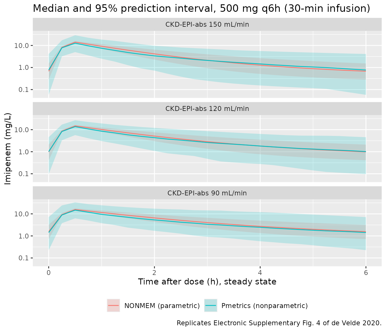
The Discussion states that “the concentrations of the 2.5th percentile are approximately twofold lower for the nonparametric model”. The table below reads the 2.5th percentile off both models at mid-interval and at trough.
p025 <- band |>
  filter(tad %in% c(3, 6)) |>
  select(model, egfr, tad, P025) |>
  pivot_wider(names_from = model, values_from = P025) |>
  mutate(Ratio = `NONMEM (parametric)` / `Pmetrics (nonparametric)`)
p025 |>
  mutate(across(where(is.numeric), ~ signif(.x, 3))) |>
  rename("Time after dose (h)" = tad, "Renal function" = egfr,
         "Ratio NONMEM / Pmetrics" = Ratio) |>
knitr::kable(caption = "2.5th percentile of simulated concentration (mg/L).")| Renal function | Time after dose (h) | NONMEM (parametric) | Pmetrics (nonparametric) | Ratio NONMEM / Pmetrics |
|---|---|---|---|---|
| CKD-EPI-abs 150 mL/min | 3 | 0.929 | 0.2500 | 3.72 |
| CKD-EPI-abs 150 mL/min | 6 | 0.282 | 0.0577 | 4.89 |
| CKD-EPI-abs 120 mL/min | 3 | 1.360 | 0.4770 | 2.84 |
| CKD-EPI-abs 120 mL/min | 6 | 0.410 | 0.0963 | 4.26 |
| CKD-EPI-abs 90 mL/min | 3 | 2.230 | 0.9090 | 2.45 |
| CKD-EPI-abs 90 mL/min | 6 | 0.718 | 0.2260 | 3.18 |
# Gate the DIRECTION only, on the median ratio across the six cells rather
# than any one cell's tail quantile (a 2.5th percentile of 200 subjects is
# the 5th-lowest value and moves between runs). The magnitude is a known
# deviation -- see the text below -- and is deliberately not gated.
stopifnot(median(p025$Ratio) > 1.5)
The direction reproduces: the nonparametric model’s lower tail sits well below the parametric one at every renal-function level. The magnitude does not. The median ratio here is 3.4, against the paper’s “approximately twofold”. The likely cause is the parametric approximation of the nonparametric arm. NPAG searched strict parameter boundaries (Ke 0-1.5 1/h, V 1-70 L, Kcp and Kpc 0-1 1/h; Sect. 3.4) and placed only 16 support points. The unbounded log-normal marginals used here, with CVs of 72-81% on the distribution rate constants, reach further into the tails than that discrete distribution can. The medians of the two models agree closely (see the NCA table below); it is the tails that differ. Use the nonparametric model for central tendency and treat its extreme percentiles with caution.
PKNCA validation
Typical subject: exact exposure identities
For a typical subject (random effects removed), the steady-state AUC
over a dosing interval must equal dose / CL and the
terminal half-life must equal the closed-form beta-phase half-life. The
reference values below are computed from the published parameters, not
from the paper’s text; the paper reports no NCA.
typ_events <- bind_rows(
  data.frame(id = 1L, time = dose_times, evid = 1L, amt = 500, rate = 1000,
             cmt = "central"),
  data.frame(id = 1L, time = c(seq(0, 96, by = 0.1), seq(96.5, 160, by = 0.5)),
             evid = 0L, amt = 0, rate = 0, cmt = "central")
) |>
  mutate(CRCL = 119) |>
  arrange(time, desc(evid))
# The last dose is at 90 h, so the tail from 96 h onward is a washout that
# PKNCA uses for the terminal half-life.

typ_sim <- bind_rows(
  rxode2::rxSolve(rxode2::zeroRe(mod_par), events = typ_events,
                  returnType = "data.frame", atol = 1e-10, rtol = 1e-10) |>
    mutate(treatment = "NONMEM"),
  rxode2::rxSolve(rxode2::zeroRe(mod_np), events = typ_events,
                  returnType = "data.frame", atol = 1e-10, rtol = 1e-10) |>
    mutate(treatment = "Pmetrics")
) |>
  mutate(id = 1L)
#> ℹ parameter labels from comments will be replaced by 'label()'
#> ℹ omega/sigma items treated as zero: 'etalkel'
#> ℹ parameter labels from comments will be replaced by 'label()'
#> ℹ omega/sigma items treated as zero: 'etalkel', 'etalk12', 'etalk21', 'etalvc', 'etae_crcl_kel'

typ_conc <- typ_sim |> filter(!is.na(Cc)) |> select(id, time, Cc, treatment)
typ_dose <- bind_rows(
  typ_events |> filter(evid == 1) |> mutate(treatment = "NONMEM"),
  typ_events |> filter(evid == 1) |> mutate(treatment = "Pmetrics")
) |>
  select(id, time, amt, treatment)

typ_int <- data.frame(start = c(90, 90), end = c(96, 160),
                      auclast = c(TRUE, FALSE), half.life = c(FALSE, TRUE))
typ_nca <- PKNCA::pk.nca(PKNCA::PKNCAdata(
  PKNCA::PKNCAconc(typ_conc, Cc ~ time | treatment + id),
  PKNCA::PKNCAdose(typ_dose, amt ~ time | treatment + id),
  intervals = typ_int
))

reference <- tibble::tibble(
  treatment = c("NONMEM", "Pmetrics"),
  auclast   = 500 / tv[, "cl"],
  half.life = tv[, "thalf_beta"]
)
cmp_typ <- nlmixr2lib::ncaComparisonTable(
  simulated = typ_nca, reference = reference, by = "treatment",
  params = c("auclast", "half.life"),
  units = c(auclast = "mg*h/L", half.life = "h"),
  tolerance_pct = 20
)
knitr::kable(cmp_typ, caption = paste(
  "Typical subject at CKD-EPI-abs 119 mL/min: PKNCA vs closed form",
  "(AUC over the steady-state interval 90-96 h = dose / CL; terminal",
  "half-life = ln 2 / beta). * marks a difference of more than 20%."
))| NCA parameter | treatment | Reference | Simulated | % diff |
|---|---|---|---|---|
| AUClast (mg*h/L) | NONMEM | 26.5 | 26.5 | -0.0% |
| AUClast (mg*h/L) | Pmetrics | 23.6 | 23.6 | -0.0% |
| t½ (h) | NONMEM | 4.76 | 4.73 | -0.4% |
| t½ (h) | Pmetrics | 2.65 | 2.64 | -0.5% |
typ_res <- as.data.frame(typ_nca) |>
  filter(PPTESTCD %in% c("auclast", "half.life")) |>
  select(treatment, PPTESTCD, PPORRES) |>
  pivot_wider(names_from = PPTESTCD, values_from = PPORRES) |>
  left_join(reference, by = "treatment", suffix = c("", "_ref"))
# Same parameters on both sides, so only numerical error separates them: the
# 90-96 h interval is 4 days into q6h dosing (>99.9% of steady state) and the
# linear-trapezoid AUC on a 0.1 h grid is within 0.5%.
stopifnot(
  all(abs(typ_res$auclast / typ_res$auclast_ref - 1) < 0.01),
  all(abs(typ_res$half.life / typ_res$half.life_ref - 1) < 0.02)
)
Virtual cohort: steady-state exposure by renal function
sim_nca <- sim |>
  filter(!is.na(Cc)) |>
  mutate(treatment = paste(sub(" .*", "", model), egfr, sep = " | ")) |>
  select(id, time, Cc, treatment)

dose_df <- bind_rows(lapply(unique(sim_nca$treatment), function(tr) {
  ids <- unique(sim_nca$id[sim_nca$treatment == tr])
  events |> filter(evid == 1, id %in% ids) |> mutate(treatment = tr)
})) |>
  select(id, time, amt, treatment)

intervals <- data.frame(start = 90, end = 96, cmax = TRUE, cmin = TRUE,
                        auclast = TRUE)
nca_res <- PKNCA::pk.nca(PKNCA::PKNCAdata(
  PKNCA::PKNCAconc(sim_nca, Cc ~ time | treatment + id),
  PKNCA::PKNCAdose(dose_df, amt ~ time | treatment + id),
  intervals = intervals
))

nca_summary <- as.data.frame(nca_res) |>
  group_by(treatment, PPTESTCD) |>
  summarise(
    value = sprintf("%.2f [%.2f-%.2f]", median(PPORRES),
                    quantile(PPORRES, 0.05), quantile(PPORRES, 0.95)),
    .groups = "drop"
  ) |>
  pivot_wider(names_from = PPTESTCD, values_from = value)
nca_summary |>
  rename("Model | renal function" = treatment,
         "Cmax (mg/L)" = cmax, "Cmin (mg/L)" = cmin,
         "AUC0-6 at SS (mg*h/L)" = auclast) |>
knitr::kable(caption = "Simulated steady-state NCA, median [5th-95th percentile], 500 mg q6h.")| Model | renal function | AUC0-6 at SS (mg*h/L) | Cmax (mg/L) | Cmin (mg/L) |
|---|---|---|---|
| NONMEM | CKD-EPI-abs 120 mL/min | 26.35 [19.37-34.70] | 14.80 [13.64-16.05] | 0.98 [0.48-1.79] |
| NONMEM | CKD-EPI-abs 150 mL/min | 22.44 [16.04-30.48] | 14.18 [12.96-15.43] | 0.68 [0.31-1.36] |
| NONMEM | CKD-EPI-abs 90 mL/min | 32.51 [23.97-44.64] | 15.73 [14.43-17.51] | 1.56 [0.79-2.96] |
| Pmetrics | CKD-EPI-abs 120 mL/min | 23.70 [8.97-50.97] | 13.69 [6.00-24.29] | 1.02 [0.18-3.53] |
| Pmetrics | CKD-EPI-abs 150 mL/min | 19.98 [7.77-48.49] | 12.69 [6.01-24.94] | 0.77 [0.11-3.31] |
| Pmetrics | CKD-EPI-abs 90 mL/min | 28.08 [12.24-68.84] | 14.76 [7.61-30.68] | 1.42 [0.34-5.49] |
# Structural check: in the NONMEM model, AUC over a steady-state interval is
# dose / CL_i with CL_i = Vc x Ke_i, so the median AUC at each renal-function
# level tracks dose / (Vc x Ke x (CRCL/119)^0.655) -- the lognormal eta has
# median 1. A mis-transcribed Ke, Vc or exponent moves this by tens of percent.
auc_par <- as.data.frame(nca_res) |>
  filter(PPTESTCD == "auclast", grepl("^NONMEM", treatment)) |>
  mutate(CRCL = as.numeric(sub(".*CKD-EPI-abs ([0-9]+).*", "\\1", treatment))) |>
  group_by(CRCL) |>
  summarise(auc_med = median(PPORRES), .groups = "drop") |>
  mutate(auc_pred = 500 / (0.637 * 29.6 * (CRCL / 119)^0.655))
knitr::kable(signif(auc_par, 4), caption = "NONMEM model: median simulated AUC0-6 vs dose / typical CL.")| CRCL | auc_med | auc_pred |
|---|---|---|
| 90 | 32.51 | 31.84 |
| 120 | 26.35 | 26.37 |
| 150 | 22.44 | 22.79 |
Assumptions and deviations
-
Re-verification against the primary.
deVelde_2020_imipenemwas first transcribed from the Zhang 2025 systematic review. Checked against this primary publication, every structural value (Ke 0.637, Kcp 0.166, Kpc 0.195, Vc 29.6, Ke(cov) 0.655, reference 119 mL/min) and the 19% IIV on Ke agree exactly. Three things changed:-
Residual error. The review labelled the NONMEM
residual “Proportional = 34.8%”. The primary fitted log-transformed
concentrations with an additive error on the log scale (Eq. 1; Table 2
“Exponential error”), so the model now uses
lnorm(expSd)withexpSd = 0.348instead ofprop(0.348). The two agree closely for small errors;lnormis the structure the authors fitted. -
Omega. The primary states the variance directly
(
omega^2 = 0.0354, Sect. 3.3), replacing the value back-calculated from the rounded 19% CV (0.0355). - Study location. The patients were treated in Geneva, Switzerland; the review listed the Netherlands, which is the authors’ affiliation. The population metadata now also carries the 30-min infusion, the 125 analysed concentrations (138 drawn, 13 below LOQ) and the renal-function summary.
-
Residual error. The review labelled the NONMEM
residual “Proportional = 34.8%”. The primary fitted log-transformed
concentrations with an additive error on the log scale (Eq. 1; Table 2
“Exponential error”), so the model now uses
-
Nonparametric arm, approximated parametrically.
NPAG estimates a discrete joint distribution (16 support points, Fig.
1), not a parametric omega matrix, and the support points are not
published. The Pmetrics model approximates that distribution with
independent log-normal marginals whose CVs match Table 2 exactly
(
omega^2 = log(CV^2 + 1)). Correlations are not reported (the paper only states none exceeded 0.95), so the marginals are independent. The approximation is required to simulate the arm at all, and it is the same treatment given to the other Pmetrics models in this package (Tsai_2023_ceftriaxone,Hughes_2024_vancomycin_nonparametric). -
Pmetrics typical values are means. Table 2 reports
the Pmetrics population by its probability-weighted mean; the model uses
each mean as the median of its log-normal marginal, following
Tsai_2023_ceftriaxone. The model’s own mean therefore sitsexp(omega^2 / 2)above the printed mean: 6% for Ke and 29% for Kcp. The bootstrap medians in Table 2 (for example Ke 0.586 1/h) are a different summary and were not used. -
Pmetrics covariate exponent is random. Eq. 10
writes the individual Ke as
Ke_i,med x (CKD-EPI-abs_i / 119)^Ke(cov)_i,med: each subject has their own exponent. The model therefore givese_crcl_kelits own log-normal eta (CV 55.2%, Table 2), in the same way asDownes_2023_vancomycin_full. -
Pmetrics residual error evaluated at the
prediction. The assay-error polynomial (Eq. 5) is evaluated at
the observation in Pmetrics and at the prediction here, which is how
nlmixr2 residual models work. The additive and proportional parts add
linearly (
combined1()), as in Eq. 3. -
Constant renal function. Both source models used
CKD-EPI-abs as a time-varying covariate (a median of three creatinine
samples per patient; NOCB in NONMEM, LOCF with interpolation in
Pmetrics). The models accept a time-varying
CRCLcolumn; the simulations above hold it constant per patient. -
Supply absolute eGFR.
CRCLhere is CKD-EPI multiplied by the patient’s BSA, in mL/min. A standard mL/min/1.73 m^2 value understates the ratio for any patient with a BSA above 1.73 m^2 (the cohort median was 1.89 m^2). - The 2.5th-percentile claim reproduces in direction, not magnitude. The Discussion’s “approximately twofold lower” for the nonparametric model comes out at roughly three- to fivefold here, because the log-normal approximation ignores the strict NPAG parameter boundaries. This is a known deviation of the approximation, not a transcription error: the medians agree, and the CVs match Table 2 exactly. Only the direction is gated.
- No erratum or correction notice for this article was found in Europe PMC (checked 2026-09-26).