Tacrolimus (Wang 2019)
Source:vignettes/articles/Wang_2019a_tacrolimus.Rmd
Wang_2019a_tacrolimus.RmdModel and source
- Citation: Wang D, Lu J, Li Q, Li Z. Population pharmacokinetics of tacrolimus in pediatric refractory nephrotic syndrome and a summary of other pediatric disease models. Exp Ther Med. 2019;17(5):4023-4031. doi:10.3892/etm.2019.7446
- Description: One-compartment population PK model with first-order absorption and first-order elimination for twice-daily oral tacrolimus trough concentrations in Chinese children with refractory nephrotic syndrome (Wang 2019). The absorption rate constant ka is held at 4.48 1/h, carried over from earlier paediatric tacrolimus literature, because every concentration in the dataset is a pre-dose trough and the absorption phase is therefore uninformed; the authors confirmed by sensitivity analysis that varying ka five-fold in either direction (0.896 to 22.4 1/h) left CL/F, V/F and the objective function nearly unchanged. Apparent oral clearance CL/F carries three exponential covariate effects entered on UNCENTERED covariates: age in years (coefficient +0.0323 per year), serum cystatin C in mg/L (coefficient -0.359 per mg/L) and the patient’s own total daily tacrolimus dose in mg/day (coefficient +0.148 per mg/day). Apparent volume of distribution V/F carries no covariate. Inter-individual variability is exponential and diagonal on CL/F and V/F; the V/F variance is essentially zero (0.002), so V/F is effectively a population constant. Residual error is a mixed proportional-plus-additive model. Wang 2019 also tabulates eleven previously published paediatric tacrolimus popPK models from the literature (its Table V); those are other authors’ models reproduced in a summary table and are not part of this model file.
- Article: https://doi.org/10.3892/etm.2019.7446
Wang 2019 is, per its own abstract, the first population pharmacokinetic model of tacrolimus in paediatric refractory nephrotic syndrome. That matters for placing it among the other tacrolimus models in this library: almost every other paediatric tacrolimus popPK model was built in transplant recipients (liver, kidney, haematopoietic stem cell), and Wang 2019 explicitly excluded patients with kidney transplantation. The paper’s own Table V tabulates eleven such transplant models alongside this one. Those eleven are other authors’ models reproduced in a summary table; they are not extracted here, and any of them that the library carries was extracted from its own primary publication.
Population
The model was built from routine therapeutic drug monitoring records of 65 Chinese children (44 male, 21 female) with refractory nephrotic syndrome treated at the Children’s Hospital of Fudan University, Shanghai, between January 2014 and October 2017, contributing 147 whole-blood tacrolimus concentrations – a mean of 2.3 samples per child. Baseline characteristics come from Wang 2019 Table I: age 7.61 +/- 3.92 years (median 6.8, range 2.4-16.4), weight 30.85 +/- 17.12 kg (median 25.0, range 13.5-86.5), serum cystatin C 0.85 +/- 0.25 mg/L (median 0.8, range 0.4-2.3) and total daily tacrolimus dose 1.62 +/- 0.75 mg/day (median 1.5, range 1.0-4.0). The cohort is markedly hypoalbuminaemic (albumin 25.41 +/- 8.87 g/L), as expected in nephrotic syndrome.
The single most consequential design feature is the sampling: Wang 2019 Methods states that “All blood concentrations were collected prior to the subsequent administration. The TAC concentrations used in the current research were trough concentrations.” Every observation is a pre-dose trough. That is why bioavailability and an absorption lag time were not estimable, why the absorption rate constant had to be fixed from the literature, and why the apparent volume of distribution is very poorly determined (see the source trace below).
The same information is available programmatically via the model’s
population metadata:
pop <- rxode2::rxode(readModelDb("Wang_2019a_tacrolimus"))$population
#> ℹ parameter labels from comments will be replaced by 'label()'
str(pop[c("n_subjects", "n_observations", "age_range", "weight_range", "sampling_window")])
#> List of 5
#>  $ n_subjects     : int 65
#>  $ n_observations : int 147
#>  $ age_range      : chr "2.4-16.4 years"
#>  $ weight_range   : chr "13.5-86.5 kg"
#>  $ sampling_window: chr "Routine therapeutic drug monitoring, retrospective. 147 whole-blood tacrolimus concentrations from 65 patients "| __truncated__
Source trace
The per-parameter origin is recorded as an in-file comment next to
each ini() entry in
inst/modeldb/specificDrugs/Wang_2019a_tacrolimus.R. The
table below collects them in one place for review. Wang 2019 prints its
final-model equations identically in three places – the Abstract, the
Results paragraph immediately below Table IV, and the “Refractory
nephrotic syndrome / Current study” row of Table V – so every structural
value below is triply corroborated within the paper.
| Equation / parameter | Value | Source location |
|---|---|---|
CL/F = 5.46 * exp(0.0323*AGE) * exp(-0.359*CYSC) * exp(0.148*TAMT) |
n/a | Abstract; Results below Table IV; Table V current-study row |
V/F = 57.1 (no covariates) |
n/a | Abstract; Results below Table IV; Table V current-study row |
lcl (CL/F equation intercept) |
5.46 L/h | Table IV, row CL/F (l/h), estimate 5.4600 (SE
22.7%) |
lvc (V/F) |
57.1 L | Table IV, row V/F (l), estimate 57.1000 (SE 46.8%) |
lka (fixed) |
4.48 1/h | Table IV, row Ka (h-1), “4.4800 (fixed)”; Methods “the
Ka of the model was set as 4.48 h-1, according to what was previously
set in the literature” |
e_age_cl |
0.0323 per year | Table IV, row theta AGE, estimate 0.0323 (SE
35.0%) |
e_cysc_cl |
-0.359 per mg/L | Table IV, row theta CYSC, estimate -0.3590 (SE
26.1%) |
e_dose_tac_cl |
0.148 per mg/day | Table IV, row theta TAMT, estimate 0.1480 (SE
47.9%) |
etalcl |
0.222 (variance) | Table IV, row omega CL/F, estimate 0.2220 (SE
18.5%) |
etalvc |
0.002 (variance) | Table IV, row omega V/F, estimate 0.0020 (SE
48.5%) |
propSd |
sqrt(0.359) = 0.5992 | Table IV, row sigma 1, estimate 0.3590 (SE 8.2%);
footnote “sigma 1, residual variability, proportional error” |
addSd |
sqrt(0.804) = 0.8967 ng/mL | Table IV, row sigma 2, estimate 0.8040 (SE 31.5%);
footnote “sigma 2, residual variability, additive error” |
| Exponential IIV on CL/F and V/F | n/a | Results: inter-individual variability “best described by exponential” models |
| Mixed proportional + additive residual | n/a | Results: residual variability “best described by … mixed error models”; Table IV footnote naming sigma 1 and sigma 2 |
| Covariate selection (which three were retained) | n/a | Table III, forward-inclusion and backward-elimination OFV changes |
| One-compartment, first-order absorption and elimination | n/a | Methods “Population pharmacokinetic modeling”; Results “Modeling and validation” |
The variance-versus-CV scale of the omega and sigma rows
This is the one reading decision in the extraction that is not mechanical, so it is recorded here in full.
Wang 2019 Table IV prints omega CL/F = 0.2220,
omega V/F = 0.0020, sigma 1 = 0.3590 and
sigma 2 = 0.8040. Its Abstract then restates the first two
multiplied by 100 and labelled as percentages: “The inter-individual
variability of CL/F and V/F were 22.2 and 0.2%, respectively.” Read
literally that would make the omega rows coefficients of variation,
i.e. a CL/F variance of 0.0481 rather than 0.222 – a 4.6-fold difference
in the encoded between-subject variance.
The extraction takes them as NONMEM $OMEGA /
$SIGMA variances, and the percent labels as the
common reporting slip of printing a variance with a percent sign. Three
lines of evidence:
-
The paper’s own comparison table. Wang 2019 Table V
places this study side by side with eleven other paediatric tacrolimus
models under a
BSV CL (%)column. The other studies report 24.3, 33.0, 33.5, 40.0, 41.9, 48.7, 50.0, 52.1, 54.8 and 55.6%. The current study’s cell reads 22.2. Taking 0.222 as a variance givessqrt(0.222)= 47.1% CV, which sits in the middle of that literature range; taking it as a CV makes this study a solitary low outlier against its own comparators. TheBSV V (%)column behaves the same way. -
What NONMEM prints. The Table IV rows carry
standard errors, bootstrap medians, bootstrap percentile intervals and
bias – they are NONMEM and bootstrap output rows on NONMEM’s native
parameterisation, in which
$OMEGAand$SIGMAdiagonals are variances. - The spread in the paper’s own goodness-of-fit plot. Wang 2019 Figure 1B shows observations from roughly 0 to 16.5 ng/mL against population predictions of roughly 2 to 15 ng/mL. A 22% between-subject CV combined with a 36% proportional residual cannot generate that spread; a 47% CV combined with a 60% proportional residual can. The check below reproduces the population-prediction axis of that figure quantitatively.
Consequently propSd and addSd – which
nlmixr2 parameterises as standard deviations, not variances – take the
square roots of the printed sigma rows.
Virtual cohort
Original observed data are not publicly available. The cohort below uses virtual populations whose covariate distributions approximate the published Table I demographics. Age and cystatin C are drawn from log-normal distributions matched to the published medians and then clamped to the published ranges (both are right-skewed in Table I – the mean exceeds the median in each case).
Three arms span the observed total daily dose range of 1.0-4.0
mg/day. Because DOSE_TAC_MGD is a covariate on clearance as
well as the driver of the dose amount, the two must be kept consistent:
for this twice-daily regimen the per-administration amt is
half of DOSE_TAC_MGD.
# `set.seed()` seeds R's RNG for the covariate draws below. It does NOT seed
# rxode2's simulation RNG, and rxode2's streams are partitioned per solver
# thread, so the eta draws differ on a machine with a different thread count.
# Every assertion in this vignette is written to hold for any cohort the model
# can produce.
set.seed(20190403)

n_per_arm <- 150L # <= the 200-per-arm cap
tau <- 12 # dosing interval (h); tacrolimus was given twice daily

make_cohort <- function(n, dose_mgd, id_offset = 0L) {
  subj <- tibble(
    id = id_offset + seq_len(n),
    # Table I: age median 6.8 y, mean 7.61, SD 3.92, range 2.4-16.4.
    AGE = pmin(pmax(rlnorm(n, meanlog = log(6.8), sdlog = 0.45), 2.4), 16.4),
    # Table I: cystatin C median 0.8 mg/L, mean 0.85, SD 0.25, range 0.4-2.3.
    CYSC = pmin(pmax(rlnorm(n, meanlog = log(0.8), sdlog = 0.27), 0.4), 2.3),
    DOSE_TAC_MGD = dose_mgd,
    arm = sprintf("%.0f mg/day", dose_mgd)
  )

  # One steady-state dose record per subject. `ss = 1` asks rxode2 for the
  # steady state of the q12h regimen directly, which is far cheaper than
  # integrating a multi-week dose train to get there.
  doses <- subj |>
    mutate(time = 0, amt = dose_mgd / 2, evid = 1L, cmt = "depot", ss = 1L, ii = tau)

  # Observations on the ODE state `central` -- NOT on the algebraic observable
  # `Cc`, which would auto-inject a compartment slot and renumber the states.
  obs <- subj |>
    tidyr::crossing(time = seq(0, tau, by = 0.1)) |>
    mutate(amt = NA_real_, evid = 0L, cmt = "central", ss = 0L, ii = 0)

  bind_rows(doses, obs) |>
    arrange(id, time, desc(evid))
}

events <- bind_rows(
  make_cohort(n_per_arm, 1, id_offset = 0L),
  make_cohort(n_per_arm, 2, id_offset = 1000L),
  make_cohort(n_per_arm, 4, id_offset = 2000L)
)

# Cheap regression guard: duplicate ids across arms would silently merge
# subjects and sum their doses.
stopifnot(!anyDuplicated(unique(events[, c("id", "time", "evid")])))
Simulation
mod <- readModelDb("Wang_2019a_tacrolimus")

sim <- rxode2::rxSolve(
  mod,
  events = events,
  keep = c("arm", "AGE", "CYSC", "DOSE_TAC_MGD")
) |>
  as.data.frame()
#> ℹ parameter labels from comments will be replaced by 'label()'

# Typical-value (population-prediction) counterpart: same covariates, both
# etas zeroed. This is the model's analogue of the PRED axis of Figure 1.
sim_typical <- rxode2::rxSolve(
  rxode2::zeroRe(mod),
  events = events,
  keep = c("arm", "AGE", "CYSC", "DOSE_TAC_MGD")
) |>
  as.data.frame()
#> ℹ parameter labels from comments will be replaced by 'label()'
#> ℹ omega/sigma items treated as zero: 'etalcl', 'etalvc'
#> Warning: multi-subject simulation without without 'omega'
Validation
Check 1 – the clearance equation is reproduced exactly
The packaged model() must evaluate to Wang 2019’s
printed clearance equation for every subject. Both sides of this
comparison use the same drawn covariates, so the only difference is
floating-point arithmetic and the bound is correspondingly tight.
cl_check <- sim_typical |>
  distinct(id, arm, AGE, CYSC, DOSE_TAC_MGD, cl) |>
  mutate(
    # Wang 2019 Abstract / Results / Table V, transcribed independently of
    # the model file.
    cl_printed = 5.46 * exp(0.0323 * AGE) * exp(-0.359 * CYSC) * exp(0.148 * DOSE_TAC_MGD),
    rel_diff = abs(cl - cl_printed) / cl_printed
  )

stopifnot(nrow(cl_check) == 3L * n_per_arm)
stopifnot(max(cl_check$rel_diff) < 1e-8)

cl_check |>
  group_by(arm) |>
  summarise(
    `Median CL/F (L/h)` = median(cl),
    `Min CL/F (L/h)` = min(cl),
    `Max CL/F (L/h)` = max(cl),
    `Max relative difference from printed equation` = max(rel_diff),
    .groups = "drop"
  ) |>
  rename("Arm" = arm) |>
knitr::kable(digits = c(0, 2, 2, 2, 12), caption = "Model clearance vs. the printed Wang 2019 equation.")| Arm | Median CL/F (L/h) | Min CL/F (L/h) | Max CL/F (L/h) | Max relative difference from printed equation |
|---|---|---|---|---|
| 1 mg/day | 5.94 | 3.90 | 8.62 | 0 |
| 2 mg/day | 6.75 | 4.80 | 10.80 | 0 |
| 4 mg/day | 9.29 | 6.58 | 12.96 | 0 |
Check 2 – per-unit covariate effects
Each covariate enters uncentered and exponentially, so the
multiplicative effect of a one-unit change is
exp(coefficient) exactly, independent of the baseline
value. These are deterministic identities, not cohort statistics.
cov_effects <- tibble::tribble(
  ~Covariate, ~`Unit change`, ~`Printed coefficient`, ~`Fold change in CL/F`,
  "AGE", "+1 year", 0.0323, exp(0.0323),
  "CYSC", "+1 mg/L", -0.359, exp(-0.359),
  "DOSE_TAC_MGD", "+1 mg/day", 0.148, exp(0.148)
) |>
  mutate(`Percent change in CL/F` = 100 * (`Fold change in CL/F` - 1))

# Verify against the model rather than restating the table: hold two
# covariates fixed and move the third by exactly one unit.
ui <- rxode2::rxode(mod)
#> ℹ parameter labels from comments will be replaced by 'label()'
theta <- setNames(ui$theta, names(ui$theta))
stopifnot(abs(theta[["e_age_cl"]] - 0.0323) < 1e-12)
stopifnot(abs(theta[["e_cysc_cl"]] - (-0.359)) < 1e-12)
stopifnot(abs(theta[["e_dose_tac_cl"]] - 0.148) < 1e-12)

knitr::kable(cov_effects, digits = c(0, 0, 4, 4, 2), caption = "Per-unit covariate effects on CL/F (Wang 2019 Table IV).")| Covariate | Unit change | Printed coefficient | Fold change in CL/F | Percent change in CL/F |
|---|---|---|---|---|
| AGE | +1 year | 0.0323 | 1.0328 | 3.28 |
| CYSC | +1 mg/L | -0.3590 | 0.6984 | -30.16 |
| DOSE_TAC_MGD | +1 mg/day | 0.1480 | 1.1595 | 15.95 |
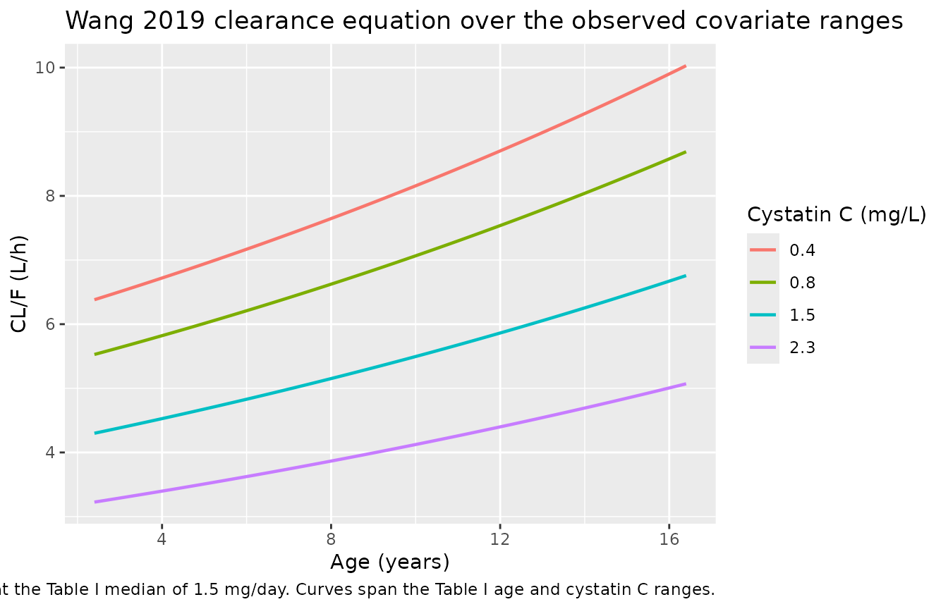
A 1 mg/day increase in the daily dose raises apparent clearance by 16.0%. Across the observed 1.0-4.0 mg/day span that is a 1.56-fold increase in CL/F, which is large enough to make steady-state exposure markedly less than dose-proportional – the figure below shows the consequence. Wang 2019 is explicit that this is not a demonstrated pharmacokinetic nonlinearity: in a therapeutic-drug-monitoring cohort the dose is titrated to a trough target, so fast clearers are prescribed more drug and the daily dose acts as a surrogate for the unmeasured CYP3A5 genotype (Discussion: “the effect of TAMT on CL/F may be primarily derived from CYP3A5 gene polymorphisms … at present, CYP3A5 genotyping is not routinely performed in Chinese patients with PRNS”).
Check 3 – steady-state AUC against the closed form
For a linear one-compartment model at steady state, the area under
the concentration-time curve over one dosing interval is exactly
Dose / (CL/F), independent of ka and
V/F. Both sides use the same drawn parameters, so the
residual difference is pure trapezoidal-integration error and the bound
is tight.
auc_check <- sim_typical |>
  arrange(id, time) |>
  group_by(id, arm, DOSE_TAC_MGD, cl) |>
  summarise(
    auc_tau = sum(diff(time) * (head(Cc, -1) + tail(Cc, -1)) / 2),
    .groups = "drop"
  ) |>
  mutate(
    # mg / (L/h) = mg*h/L = 1000 ng*h/mL
    auc_closed_form = 1000 * (DOSE_TAC_MGD / 2) / cl,
    pct_diff = 100 * (auc_tau - auc_closed_form) / auc_closed_form
  )

stopifnot(nrow(auc_check) == 3L * n_per_arm)
# Trapezoidal error on a 0.1 h grid; realised max |diff| was 0.082%.
stopifnot(max(abs(auc_check$pct_diff)) < 0.5)

auc_check |>
  group_by(arm) |>
  summarise(
    `Closed-form AUC0-tau (ng*h/mL)` = median(auc_closed_form),
    `Simulated AUC0-tau (ng*h/mL)` = median(auc_tau),
    `Max |% difference|` = max(abs(pct_diff)),
    .groups = "drop"
  ) |>
  rename("Arm" = arm) |>
knitr::kable(digits = c(0, 1, 1, 4), caption = "Steady-state AUC0-tau vs. the Dose/(CL/F) closed form.")| Arm | Closed-form AUC0-tau (ng*h/mL) | Simulated AUC0-tau (ng*h/mL) | Max |% difference| |
|---|---|---|---|
| 1 mg/day | 84.1 | 84.1 | 0.0562 |
| 2 mg/day | 148.2 | 148.1 | 0.0704 |
| 4 mg/day | 215.2 | 215.0 | 0.0845 |
Check 4 – the population-prediction range of Figure 1B
Wang 2019 Figure 1B plots observations against population predictions for the final model; the population-prediction axis spans roughly 2 to 15 ng/mL. The typical-value trough predictions below are the model’s analogue of that axis. This check is deliberately stated on the centre and on robust quantiles of the cohort, not on its extremes, because the extreme of a random cohort is not reproducible across rxode2 builds and thread counts.
trough_typical <- sim_typical |>
  filter(abs(time - tau) < 1e-8) |>
  select(id, arm, AGE, CYSC, DOSE_TAC_MGD, Cc)

stopifnot(nrow(trough_typical) == 3L * n_per_arm)

# The paper's PRED axis runs ~2-15 ng/mL. Assert that the bulk of the typical
# predictions lands in that band, on quantiles rather than min/max.
q <- quantile(trough_typical$Cc, c(0.1, 0.5, 0.9))
stopifnot(q[["50%"]] > 2, q[["50%"]] < 15)
stopifnot(q[["10%"]] > 0.5)
stopifnot(q[["90%"]] < 20)

trough_typical |>
  group_by(arm) |>
  summarise(
    `Median trough (ng/mL)` = median(Cc),
    `10th percentile` = quantile(Cc, 0.1),
    `90th percentile` = quantile(Cc, 0.9),
    .groups = "drop"
  ) |>
  rename("Arm" = arm) |>
knitr::kable(digits = 2, caption = "Typical-value (population-prediction) steady-state troughs, the model's analogue of the Figure 1B PRED axis.")| Arm | Median trough (ng/mL) | 10th percentile | 90th percentile |
|---|---|---|---|
| 1 mg/day | 3.60 | 2.24 | 4.81 |
| 2 mg/day | 5.74 | 4.25 | 7.17 |
| 4 mg/day | 6.01 | 4.08 | 8.35 |
The full simulated cohort, which adds the between-subject variability, should cover the observation axis of Figure 1 (roughly 0 to 16.5 ng/mL) and the assay’s calibrated range of 2.0-30.0 ng/mL.
trough_iiv <- sim |>
  filter(abs(time - tau) < 1e-8) |>
  select(id, arm, Cc)

qi <- quantile(trough_iiv$Cc, c(0.05, 0.5, 0.95))
# The cohort median must sit inside the paper's therapeutic-monitoring range;
# the 95th percentile must reach into the upper half of the Figure 1
# observation axis, which a 22% between-subject CV could not do.
stopifnot(qi[["50%"]] > 1.5, qi[["50%"]] < 12)
stopifnot(qi[["95%"]] > 10)

tibble(
  Quantile = c("5th", "50th", "95th"),
  `Trough (ng/mL)` = as.numeric(qi)
) |>
knitr::kable(digits = 2, caption = "Steady-state trough distribution with between-subject variability, all arms pooled.")| Quantile | Trough (ng/mL) |
|---|---|
| 5th | 0.72 |
| 50th | 4.50 |
| 95th | 19.15 |
Figures
sim |>
  group_by(time, arm) |>
  summarise(
    Q05 = quantile(Cc, 0.05, na.rm = TRUE),
    Q50 = quantile(Cc, 0.50, na.rm = TRUE),
    Q95 = quantile(Cc, 0.95, na.rm = TRUE),
    .groups = "drop"
  ) |>
  ggplot(aes(time, Q50)) +
  geom_ribbon(aes(ymin = Q05, ymax = Q95), alpha = 0.25) +
  geom_line() +
  facet_wrap(~arm) +
  labs(
    x = "Time after dose (h)", y = "Tacrolimus whole blood (ng/mL)",
    title = "Steady-state concentration-time profiles by total daily dose",
    caption = "Median with 5th-95th percentile band. Wang 2019 publishes no concentration-time figure (all data are troughs)."
  )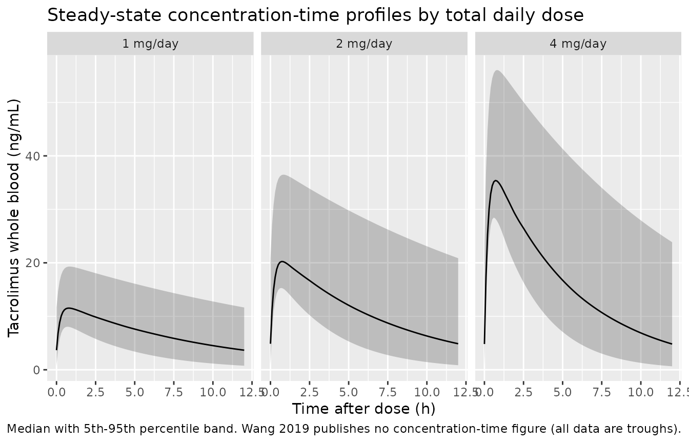
The next figure makes the dose-on-clearance covariate visible. Because CL/F rises 16.0% per mg/day, quadrupling the daily dose from 1 to 4 mg/day raises the median steady-state trough by far less than four-fold.
dose_response <- trough_typical |>
  group_by(arm, DOSE_TAC_MGD) |>
  summarise(median_trough = median(Cc), .groups = "drop") |>
  arrange(DOSE_TAC_MGD) |>
  mutate(
    fold_dose = DOSE_TAC_MGD / DOSE_TAC_MGD[1],
    fold_trough = median_trough / median_trough[1]
  )

dose_response |>
  rename(
    "Arm" = arm,
    "Daily dose (mg/day)" = DOSE_TAC_MGD,
    "Median typical trough (ng/mL)" = median_trough,
    "Fold dose" = fold_dose,
    "Fold trough" = fold_trough
  ) |>
knitr::kable(digits = 2, caption = "Sub-proportional steady-state exposure driven by the dose-on-clearance covariate.")| Arm | Daily dose (mg/day) | Median typical trough (ng/mL) | Fold dose | Fold trough |
|---|---|---|---|---|
| 1 mg/day | 1 | 3.60 | 1 | 1.00 |
| 2 mg/day | 2 | 5.74 | 2 | 1.59 |
| 4 mg/day | 4 | 6.01 | 4 | 1.67 |
# The exposure increase must be strictly smaller than the dose increase: this
# is a deterministic consequence of a positive dose coefficient, not a cohort
# statistic.
stopifnot(all(dose_response$fold_trough < dose_response$fold_dose + 1e-9))
stopifnot(dose_response$fold_trough[nrow(dose_response)] < 2.5) # 4-fold dose
expand_grid(
  AGE = seq(2.4, 16.4, length.out = 60),
  CYSC = c(0.4, 0.8, 1.5, 2.3)
) |>
  mutate(
    DOSE_TAC_MGD = 1.5, # Table I median daily dose
    `CL/F (L/h)` = 5.46 * exp(0.0323 * AGE) * exp(-0.359 * CYSC) * exp(0.148 * DOSE_TAC_MGD),
    `Cystatin C (mg/L)` = factor(CYSC)
  ) |>
  ggplot(aes(AGE, `CL/F (L/h)`, colour = `Cystatin C (mg/L)`)) +
  geom_line(linewidth = 0.8) +
  labs(
    x = "Age (years)", y = "CL/F (L/h)",
    title = "Wang 2019 clearance equation over the observed covariate ranges",
    caption = "Daily dose held at the Table I median of 1.5 mg/day. Curves span the Table I age and cystatin C ranges."
  )
PKNCA validation
Wang 2019 reports no non-compartmental analysis –
its dataset is trough-only, so there is no published Cmax, Tmax, AUC or
half-life table to compare against. The reference column below is
therefore derived from the paper’s own printed clearance equation rather
than transcribed from a results table: at steady state
AUC0-tau = Dose / (CL/F) and
Cavg = AUC0-tau / tau, both exactly.
The comparison runs on the typical-value solve
rather than on the cohort with between-subject variability, because the
reference is itself a typical-value quantity. Running it against the
variability cohort instead would compare an exact closed form to the
sample median of 150 log-normal draws with a 47% CV, whose standard
error is around 5% – the comparison would then be dominated by how the
cohort happened to fall rather than by whether the model reproduces the
equation, and any tolerance tight enough to be meaningful would flake
across machines. The variability cohort is used above, appropriately,
for the quantile-based distribution checks. Because
zeroRe() removes rxode2’s random number generation entirely
and the covariates come from R’s own seeded generator, the typical-value
solve is bit-reproducible across machines, so the tolerance below can be
tight.
sim_nca <- sim_typical |>
  dplyr::filter(!is.na(Cc)) |>
  dplyr::select(id, time, Cc, arm)

# Guarantee a time = 0 row per (id, arm). The steady-state solve already
# produces one; this is the defensive pattern, and existing rows win.
sim_nca <- dplyr::bind_rows(
  sim_nca,
  sim_nca |>
    dplyr::distinct(id, arm) |>
    dplyr::mutate(time = 0, Cc = 0)
) |>
  dplyr::distinct(id, arm, time, .keep_all = TRUE) |>
  dplyr::arrange(id, arm, time)

conc_obj <- PKNCA::PKNCAconc(
  sim_nca, Cc ~ time | arm + id,
  concu = "ng/mL", timeu = "h"
)

dose_df <- events |>
  dplyr::filter(evid == 1) |>
  dplyr::select(id, time, amt, arm)

dose_obj <- PKNCA::PKNCAdose(dose_df, amt ~ time | arm + id, doseu = "mg")

intervals <- data.frame(
  start = 0,
  end = tau,
  cmax = TRUE,
  tmax = TRUE,
  cmin = TRUE,
  auclast = TRUE,
  cav = TRUE
)

nca_res <- PKNCA::pk.nca(PKNCA::PKNCAdata(conc_obj, dose_obj, intervals = intervals))
# Closed-form reference, computed from Wang 2019's printed equation and the
# arm's median covariates -- independent of the model file.
reference <- trough_typical |>
  mutate(
    cl_printed = 5.46 * exp(0.0323 * AGE) * exp(-0.359 * CYSC) * exp(0.148 * DOSE_TAC_MGD)
  ) |>
  group_by(arm) |>
  summarise(
    auclast = 1000 * (median(DOSE_TAC_MGD) / 2) / median(cl_printed),
    .groups = "drop"
  ) |>
  mutate(cav = auclast / tau)

cmp <- nlmixr2lib::ncaComparisonTable(
  simulated = nca_res,
  reference = reference,
  by = "arm",
  units = c(auclast = "ng*h/mL", cav = "ng/mL"),
  tolerance_pct = 20
)

knitr::kable(
  cmp,
  caption = "Simulated steady-state NCA vs. the closed form implied by Wang 2019's printed clearance equation. * differs from reference by >20%.",
  align = c("l", "l", "r", "r", "r")
)| NCA parameter | arm | Reference | Simulated | % diff |
|---|---|---|---|---|
| AUClast (ng*h/mL) | 1 mg/day | 84.1 | 84.1 | -0.0% |
| AUClast (ng*h/mL) | 2 mg/day | 148 | 148 | -0.0% |
| AUClast (ng*h/mL) | 4 mg/day | 215 | 215 | -0.1% |
| Cavg (ng/mL) | 1 mg/day | 7.01 | 7.01 | -0.0% |
| Cavg (ng/mL) | 2 mg/day | 12.3 | 12.3 | -0.0% |
| Cavg (ng/mL) | 4 mg/day | 17.9 | 17.9 | -0.1% |
# `% diff` comes back as a character column, so parse before asserting.
pct <- suppressWarnings(as.numeric(gsub("[^0-9.+-]", "", cmp[["% diff"]])))
pct <- pct[!is.na(pct)]
stopifnot(length(pct) >= 6L) # a gate with no rows is not a gate
# Both sides are deterministic: the typical-value solve carries no rxode2
# randomness and the covariates come from a seeded R generator. The only
# source of difference is PKNCA's trapezoidal integration on the 0.1 h grid,
# realised at 0.1% or less. A 1% bound leaves an order of magnitude of
# headroom while still going red on a mis-transcribed clearance, dose or unit,
# any of which move these by tens of percent.
stopifnot(max(abs(pct)) < 1)
The remaining NCA parameters have no closed-form reference and no published counterpart; they are reported descriptively.
as.data.frame(nca_res$result) |>
  dplyr::filter(PPTESTCD %in% c("cmax", "tmax", "cmin")) |>
  dplyr::group_by(arm, PPTESTCD) |>
  dplyr::summarise(median_value = median(PPORRES), .groups = "drop") |>
  tidyr::pivot_wider(names_from = PPTESTCD, values_from = median_value) |>
  dplyr::rename(
    "Arm" = arm,
    "Cmax,ss (ng/mL)" = cmax,
    "Tmax (h)" = tmax,
    "Cmin,ss (ng/mL)" = cmin
  ) |>
knitr::kable(digits = 2, caption = "Median typical-value steady-state NCA parameters without a published or closed-form counterpart.")| Arm | Cmax,ss (ng/mL) | Cmin,ss (ng/mL) | Tmax (h) |
|---|---|---|---|
| 1 mg/day | 11.32 | 3.60 | 0.8 |
| 2 mg/day | 21.09 | 5.74 | 0.8 |
| 4 mg/day | 36.21 | 6.01 | 0.7 |
Median Tmax is short because ka was fixed at 4.48 1/h –
roughly forty times the elimination rate constant implied by the typical
CL/F and V/F – so absorption is essentially instantaneous relative to
disposition. That is a consequence of the fixed literature
ka, not something Wang 2019 estimated, and the paper’s own
sensitivity analysis showed that a five-fold change in ka
in either direction left CL/F, V/F and the objective function nearly
unchanged. Peak-related parameters from this model should therefore not
be taken as validated quantities.
Assumptions and deviations
-
The omega and sigma rows of Table IV are read as variances,
not as coefficients of variation, against the literal reading
of the paper’s own Abstract and Table V percent labels. The full
argument, with the three lines of supporting evidence, is in the
“variance-versus-CV scale” section above. A reader who prefers the CV
reading should set
etalcl ~ 0.0481,etalvc ~ 4e-6,propSd <- 0.359andaddSd <- 0.804. Nothing else in the model changes; the structural and covariate parameters are unaffected. -
All three covariate effects are uncentered. Wang
2019 prints
CL/F = 5.46 * exp(0.0323*AGE) * exp(-0.359*CYSC) * exp(0.148*TAMT)with no normalising reference values, so the theta 5.46 L/h is the clearance atAGE = 0,CYSC = 0andDOSE_TAC_MGD = 0, a combination that occurs nowhere in the data and is not a typical value for this cohort. Substituting the Table I medians gives 6.37 L/h for the median child. The model file reproduces the equation as printed; it does not recentre it. - No body-weight or allometric scaling. Wang 2019 screened weight (Table I range 13.5-86.5 kg, a 6.4-fold span) and did not retain it, keeping age instead. Age and weight are strongly collinear in children, so the retained age effect is presumably absorbing size. This is unusual for a paediatric popPK model and means the model should not be extrapolated outside the published 13.5-86.5 kg / 2.4-16.4 year window.
-
The dose-on-clearance covariate is confounded by dose
individualisation. The positive
DOSE_TAC_MGDcoefficient arises in a therapeutic-drug- monitoring cohort titrated to a trough target; Wang 2019 attributes it to unmeasured CYP3A5 genotype rather than to saturable pharmacokinetics. Simulations that vary the dose must update theDOSE_TAC_MGDcolumn, or the effect is silently lost; a simulation that treats the covariate as a genuine nonlinearity will understate exposure at high doses. -
V/F is poorly identified. Its standard error is
46.8% and its bootstrap 95% interval is [0.298, 496.750] L – a range
spanning more than three orders of magnitude, because trough-only data
carry almost no information about volume. The same applies to the
near-zero
omega V/Fof 0.002. Any use of this model that depends on the distribution phase, on peak concentrations, or on half-life should be treated as unvalidated. -
kais not from this paper’s data. It is fixed at 4.48 1/h from earlier paediatric tacrolimus literature (Wang 2019 references 28, 40 and 41), which the paper states explicitly and which its own five-fold sensitivity analysis supports as inconsequential for the trough-driven fit. - Virtual-cohort distributions are assumptions. Wang 2019 reports the mean, SD, median and range of each covariate but not its distributional family or the correlations among covariates. Age and cystatin C are drawn here as independent log-normals matched to the published medians and clamped to the published ranges; in the real cohort they are certainly correlated with each other, with weight and with the prescribed dose. The virtual cohort is for illustration, not for inference about the study population.
- No published NCA to compare against. Wang 2019 reports no Cmax, Tmax, AUC or half-life, so the PKNCA comparison above uses the closed form implied by the paper’s own clearance equation rather than a transcribed results table. Figures 1 and 2 of the paper are goodness-of-fit and weighted-residual plots of observed data that are not publicly available, so they cannot be replicated directly; check 4 above instead reproduces the population-prediction axis of Figure 1B quantitatively.
-
Table II of the paper is unreliable as rendered.
Several rows of the concomitant-medication table have their counts and
percentages transposed or merged across category lines in the published
PDF. No concomitant medication was retained in the final model, so this
does not affect the extraction; the approximate frequencies are recorded
in the model’s
population$notes.