RSV vaccine immune correlates of protection (Kashihara 2026)
Source:vignettes/articles/Kashihara_2026_rsvVaccine_immune_correlates.Rmd
Kashihara_2026_rsvVaccine_immune_correlates.RmdModel and source
- Citation: Kashihara Y, Qin L, Shimizu S, Diderichsen PM, Kotsuma M, Yoshihara K. Establishing Immune Correlates of Protection Against Respiratory Syncytial Virus Infection to Accelerate Vaccine Development: A Model-Based Meta-Analysis. CPT Pharmacometrics Syst Pharmacol. 2026;15:e70133. doi:10.1002/psp4.70133.
- Article: https://doi.org/10.1002/psp4.70133
This paper is a model-based meta-analysis (MBMA),
not a population PK analysis. The unit of observation is a published
trial-level vaccine efficacy, and the model is a weighted linear
mixed-effects meta-regression (R nlme) with no time course,
no dosing and no concentrations. There is therefore no PKNCA section in
this vignette; the validation below replaces it with structural checks,
exact replication of the paper’s own published predictions, and a
between-trial variability check.
The paper reports two models, which are extracted as two files:
| Model file | Paper’s role | What it adds |
|---|---|---|
Kashihara_2026_rsvVaccine_sna_mbma |
Primary analysis (Table 3 upper block, CCA, RSV-A SNA; Figure 1) | Severity-specific intercept and slope on SNA |
Kashihara_2026_rsvVaccine_snaCmi_mbma |
Secondary exploratory analysis (Table 3 lower block, MI, RSV-A SNA; Figure 3) | One common SNA slope, plus an interferon-gamma slope on LRTD 3+ only |
mod_sna    <- readModelDb("Kashihara_2026_rsvVaccine_sna_mbma")
mod_snacmi <- readModelDb("Kashihara_2026_rsvVaccine_snaCmi_mbma")

# Typical-value (zeroRe) copies for every deterministic replication below.
# The between-trial variability check further down deliberately uses the
# unmodified model instead.
tv_sna    <- rxode2::zeroRe(mod_sna)
#> ℹ parameter labels from comments will be replaced by 'label()'
tv_snacmi <- rxode2::zeroRe(mod_snacmi)
#> ℹ parameter labels from comments will be replaced by 'label()'
Population
The analysis pooled seven randomised, placebo-controlled phase 2b and later trials in older adults, together enrolling 132,677 participants (Kashihara 2026 Table 1). Six trials enrolled adults aged 60 years and older; CYPRESS enrolled adults aged 65 years and older. Every trial gave a single dose of vaccine or placebo and covered a single RSV season, from fall to the end of spring. The seven trials used seven different vaccines spanning four platforms: adjuvanted protein subunit (RSVpreF3 with AS01E in AReSVi-006; MEDI-7510 with glucopyranosyl lipid adjuvant in D4420C00005), unadjuvanted protein subunit (RSVpreF in RENOIR; RSV F in Resolve), mRNA (mRNA-1345 in ConquerRSV), and viral vector (Ad26.RSV.preF in CYPRESS; MVA-BN-RSV in VANIR).
Because the trials are the observations, the “population” of this model is a population of trials. Efficacy is reported at three clinical severity levels: RSV acute respiratory infection (ARI), RSV lower respiratory tract disease with at least two clinical symptoms (LRTD 2+), and with at least three (LRTD 3+). Endpoint definitions differed slightly between trials and were mapped onto these three levels by the authors (Kashihara 2026 Table 1 footnotes a-d).
The same information is available programmatically via
readModelDb("Kashihara_2026_rsvVaccine_sna_mbma")()$population.
Source trace
Per-parameter origins are recorded as in-file comments beside each
ini() entry in
inst/modeldb/specificDrugs/Kashihara_2026_rsvVaccine_sna_mbma.R
and ..._snaCmi_mbma.R. They are collected here for
review.
Equations
| Equation | Source location |
|---|---|
-log(1 - VE_ik/100) = Intercept_k + Slope_k * SNA_i + eta_i + eps_ik |
Kashihara 2026 Equation 1 |
SNA_i = log2(SNA_vaccine,i) - log2(SNA_placebo,i) |
Kashihara 2026 Equation 2 |
-log(1 - VE_ik/100) = Intercept_k + Slope_k * SNA_i + Slope_IFN,k * CMI_i + eta_i + eps_ik |
Kashihara 2026 Equation 3 |
CMI_i = ln(IFNg_vaccine,i) - ln(IFNg_placebo,i) |
Kashihara 2026 Equation 4 |
VE = 100 * (1 - exp[-(Intercept + Slope * SNA)]) |
Kashihara 2026 Methods 2.2.1, back-transformation |
Note the deliberately different log bases: base 2 for SNA (Equation 2) and natural log for interferon-gamma (Equation 4).
Primary model parameters
(Kashihara_2026_rsvVaccine_sna_mbma)
All from Kashihara 2026 Table 3, SNA-VE model block,
columns headed
RSV-A SNA / Primary analysis based on CCA approach.
| Parameter | Value | SE | 95% CI | Source row |
|---|---|---|---|---|
tve_ref_ari |
0.047 | 0.296 | [-0.531, 0.626] | RSV-ARI intercept |
tve_ref_lrtd2 |
-0.121 | 0.296 | [-0.700, 0.458] | RSV-LRTD2+ intercept |
tve_ref_lrtd3 |
-0.293 | 0.297 | [-0.874, 0.287] | RSV-LRTD3+ intercept |
e_sna_tve_ari |
0.323 | 0.110 | [0.109, 0.537] | SNA slope on RSV-ARI |
e_sna_tve_lrtd2 |
0.285 | 0.110 | [0.070, 0.501] | SNA slope on RSV-LRTD2+ |
e_sna_tve_lrtd3 |
0.517 | 0.117 | [0.289, 0.745] | SNA slope on RSV-LRTD3+ |
eta_study_tve |
0.315 (SD); 0.099225 (variance) | - | - | Between-trial variability (SD) |
Secondary model parameters
(Kashihara_2026_rsvVaccine_snaCmi_mbma)
All from Kashihara 2026 Table 3, SNA + CMI-VE model
block, columns headed RSV-A SNA / MI approach. The adjacent
CCA approach columns are the model development step and are
reproduced in the last column for reference only; they are
not what the model file encodes (see Assumptions and
deviations).
| Parameter | Value (MI, encoded) | SE | 95% CI | Source row | CCA value (not encoded) |
|---|---|---|---|---|---|
tve_ref_ari |
0.051 | 0.247 | [-0.490, 0.591] | RSV-ARI intercept | 0.150 |
tve_ref_lrtd2 |
-0.168 | 0.247 | [-0.709, 0.373] | RSV-LRTD2+ intercept | -0.069 |
tve_ref_lrtd3 |
-0.298 | 0.309 | [-1.02, 0.425] | RSV-LRTD3+ intercept | -0.573 |
e_sna_tve |
0.321 | 0.091 | [0.120, 0.521] | SNA slope | 0.256 |
e_ifng_tve_lrtd3 |
0.111 | 0.138 | [-2.00, 2.23] | IFN-g slope on RSV-LRTD3+ | 0.418 |
eta_study_tve |
0.318 (SD); 0.101124 (variance) | - | - | Between-trial variability (SD) | 0.382 |
Analysis dataset
The paper’s analysis dataset is small enough to reproduce in full. This is Kashihara 2026 Table 2 verbatim: VE with its 95% confidence interval at each severity level, and the immunogenicity readouts as ratios to placebo on the original scale (Table 2 footnote b).
tab2 <- tibble::tribble(
  ~study,        ~sna_a, ~sna_b, ~ifng, ~cd4,
  "AReSVi-006",    10.7,    8.1,    NA,  8.3,
  "ConquerRSV",     7.7,    9.8,    NA,   NA,
  "CYPRESS",       13.0,   10.3,  12.8,   NA,
  "D4420C00005",    2.5,     NA,   9.0,   NA,
  "RENOIR",        13.9,   12.8,  20.6,  2.5,
  "Resolve",        1.6,    1.4,    NA,   NA,
  "VANIR",          1.6,    1.5,   3.5,   NA
)

ve_obs <- tibble::tribble(
  ~study,        ~severity,  ~ve,   ~lo,     ~hi,
  "AReSVi-006",  "ARI",      71.7,   56.2,   82.3,
  "AReSVi-006",  "LRTD 2+",  82.6,   57.9,   94.1,
  "AReSVi-006",  "LRTD 3+",  94.1,   62.4,   99.9,
  "ConquerRSV",  "ARI",      68.4,   50.9,   79.7,
  "ConquerRSV",  "LRTD 2+",  83.7,   66.1,   92.2,
  "ConquerRSV",  "LRTD 3+",  82.4,   34.8,   95.3,
  "CYPRESS",     "ARI",      69.8,   43.7,   84.7,
  "CYPRESS",     "LRTD 2+",  75.0,   50.1,   88.5,
  "CYPRESS",     "LRTD 3+",  80.0,   52.2,   92.9,
  "D4420C00005", "ARI",      -7.1, -106.9,   44.3,
  "D4420C00005", "LRTD 2+", -36.9, -188.2,   33.5,
  "RENOIR",      "ARI",      62.1,   37.1,   77.9,
  "RENOIR",      "LRTD 2+",  66.7,   28.8,   85.8,
  "RENOIR",      "LRTD 3+",  85.7,   32.0,   98.7,
  "Resolve",     "ARI",      12.6,  -14.0,   33.0,
  "Resolve",     "LRTD 3+",   -7.9,  -84.0,  37.0,
  "VANIR",       "ARI",      48.8,   25.8,   64.7,
  "VANIR",       "LRTD 2+",  59.0,   34.7,   74.3,
  "VANIR",       "LRTD 3+",  42.9,  -16.1,   71.9
) |>
  mutate(severity = factor(severity, levels = c("ARI", "LRTD 2+", "LRTD 3+")))
Dataset structural checks
Two counts stated in the paper’s own text are exact, independent checks that the table above was transcribed correctly. Both are free regression tests: a single mis-keyed or dropped row breaks them.
# Kashihara 2026 Results 3.2: "A total of 19 VE values across seven studies
# were included in the analysis."
n_ve_primary    <- nrow(ve_obs)
n_study_primary <- dplyr::n_distinct(ve_obs$study)

# Kashihara 2026 Results 3.3: "A total of 11 VE values across four studies
# were included in the CCA" -- the complete-case set for the secondary model
# is the studies with an OBSERVED interferon-gamma value.
cca_studies  <- tab2$study[!is.na(tab2$ifng)]
n_ve_cca     <- sum(ve_obs$study %in% cca_studies)
n_study_cca  <- length(cca_studies)

stopifnot(
  n_ve_primary    == 19L,
  n_study_primary ==  7L,
  n_ve_cca        == 11L,
  n_study_cca     ==  4L
)

# Guard against a vacuous pass: the LRTD 3+ level must actually be missing for
# D4420C00005 and LRTD 2+ for Resolve, which is why 19 and not 21.
stopifnot(
  !any(ve_obs$study == "D4420C00005" & ve_obs$severity == "LRTD 3+"),
  !any(ve_obs$study == "Resolve"     & ve_obs$severity == "LRTD 2+"),
  # Kashihara 2026 Results 3.1: "Only two studies reported or could be cross
  # matched for CD4+ T cells data."
  sum(!is.na(tab2$cd4)) == 2L,
  # Discussion: "The small number of observed IFN-gamma data points (n = 4)".
  sum(!is.na(tab2$ifng)) == 4L
)

c(n_ve_primary = n_ve_primary, n_study_primary = n_study_primary,
  n_ve_cca = n_ve_cca, n_study_cca = n_study_cca)
#>    n_ve_primary n_study_primary        n_ve_cca     n_study_cca
#>              19               7              11               4
Simulation helper
The models are static: one row in, one prediction out. No dosing
records and no time course are needed, so a single evid = 0
row per scenario is the whole event table.
# Solve either model over a grid of immunogenicity values. `IFNG_PBORATIO` is
# supplied to both models, but rxode2 returns a covariate column only when the
# model actually references it -- the SNA-only model does not, so that column
# comes back for the secondary model and not the primary one. `any_of()`
# tolerates both shapes; a fixed `select()` would error on the primary model.
solve_grid <- function(model, sna_ratio, ifng_ratio = 1) {
  ev <- expand.grid(SNA_RSVA_PBORATIO = sna_ratio, IFNG_PBORATIO = ifng_ratio)
  ev$id   <- seq_len(nrow(ev))
  ev$time <- 0
  ev$amt  <- 0
  ev$evid <- 0
  out <- rxode2::rxSolve(model, ev, returnType = "data.frame") |>
    dplyr::select(dplyr::any_of(c("SNA_RSVA_PBORATIO", "IFNG_PBORATIO")),
                  ve_ari, ve_lrtd2, ve_lrtd3,
                  tve_ari, tve_lrtd2, tve_lrtd3)
  # One prediction row per input scenario: guards against a silent endpoint
  # fan-out or an id collision.
  stopifnot(nrow(out) == nrow(ev))
  out
}
Back-transformation check
A dimensional-analysis-style check that the model’s
model() block implements the paper’s back-transformation
exactly, and that the intercepts mean what the paper says they mean. At
an SNA ratio of 1 the vaccine and placebo arms have equal titers, so
log2(1) = 0 and the linear predictor collapses to the
intercept alone.
at_unity <- solve_grid(tv_sna, sna_ratio = 1)
#> ℹ omega/sigma items treated as zero: 'eta_study_tve'

intercepts <- c(ARI = 0.047, `LRTD 2+` = -0.121, `LRTD 3+` = -0.293)
expected   <- 100 * (1 - exp(-intercepts))
observed   <- c(at_unity$ve_ari, at_unity$ve_lrtd2, at_unity$ve_lrtd3)

# Deterministic arithmetic: a tight bound is correct here and is the point.
stopifnot(max(abs(observed - expected)) < 1e-8)

# Kashihara 2026 Results 3.2: "Intercepts represented the VE when SNA levels
# were equal between vaccinated and placebo groups. In this case, similar
# infection rates in both groups would result in theoretical VE close to
# zero, which explains the lack of statistical significance of the intercept
# parameters." Each reported 95% CI spans zero, which is the paper's own
# statement of that claim; assert it on the transcribed intervals.
ci <- tibble::tribble(
  ~severity,  ~lo,    ~hi,
  "ARI",      -0.531, 0.626,
  "LRTD 2+",  -0.700, 0.458,
  "LRTD 3+",  -0.874, 0.287
)
stopifnot(all(ci$lo < 0 & ci$hi > 0))

tibble(severity = names(intercepts), intercept = intercepts,
       ve_at_ratio_1 = round(observed, 1))
#> # A tibble: 3 × 3
#>   severity intercept ve_at_ratio_1
#>   <chr>        <dbl>         <dbl>
#> 1 ARI          0.047           4.6
#> 2 LRTD 2+     -0.121         -12.9
#> 3 LRTD 3+     -0.293         -34
Replicate Figure 1: SNA vs vaccine efficacy
Figure 1 of Kashihara 2026 plots the typical-value VE against the RSV-A SNA ratio at each of the three severity levels, with the observed trial VE values and their 95% confidence intervals overlaid.
grid_sna <- solve_grid(tv_sna, sna_ratio = exp(seq(log(1), log(20), length.out = 120)))
#> ℹ omega/sigma items treated as zero: 'eta_study_tve'
#> Warning: multi-subject simulation without without 'omega'

pred_long <- grid_sna |>
  select(SNA_RSVA_PBORATIO, ve_ari, ve_lrtd2, ve_lrtd3) |>
  pivot_longer(-SNA_RSVA_PBORATIO, names_to = "key", values_to = "ve") |>
  mutate(severity = factor(
    recode(key, ve_ari = "ARI", ve_lrtd2 = "LRTD 2+", ve_lrtd3 = "LRTD 3+"),
    levels = c("ARI", "LRTD 2+", "LRTD 3+")
  ))

obs_plot <- ve_obs |> left_join(tab2 |> select(study, sna_a), by = "study")

ggplot(pred_long, aes(SNA_RSVA_PBORATIO, ve)) +
  geom_hline(yintercept = 0, linewidth = 0.3, colour = "grey60") +
  geom_line(linewidth = 0.9, colour = "#2166ac") +
  geom_errorbar(data = obs_plot,
                aes(x = sna_a, y = ve, ymin = lo, ymax = hi),
                width = 0.05, colour = "grey35", linewidth = 0.35) +
  geom_point(data = obs_plot, aes(x = sna_a, y = ve),
             colour = "black", size = 1.6) +
  facet_wrap(~severity) +
  scale_x_log10(breaks = c(1, 2, 5, 10, 20)) +
  coord_cartesian(ylim = c(-100, 100)) +
  labs(x = "RSV-A SNA (ratio to placebo)", y = "Vaccine efficacy (%)",
       caption = paste("Replicates Figure 1 of Kashihara 2026.",
                       "Line: typical-value prediction. Points and bars:",
                       "observed VE and 95% CI (Table 2)."))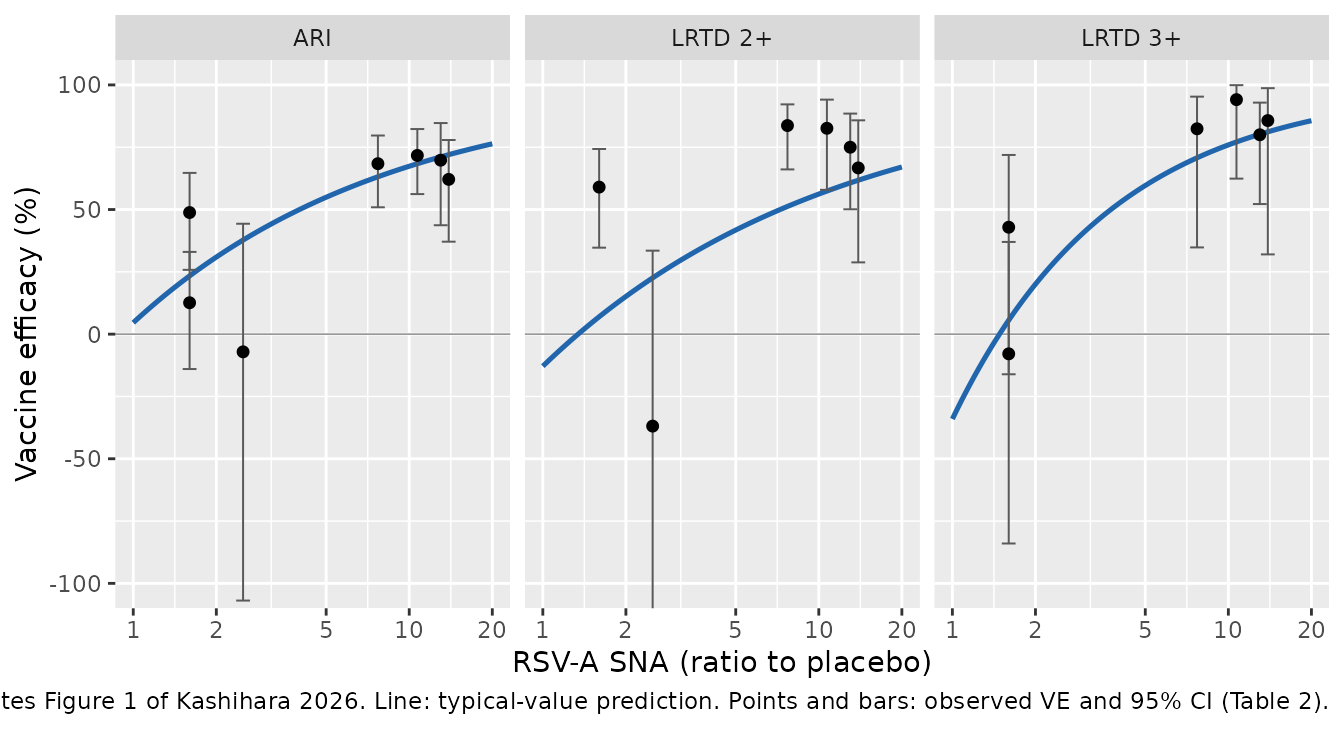
The paper’s headline prediction
Kashihara 2026 states the correlate twice in numeric form:
“a ratio of RSV-A SNA titer to placebo of eight would correspond to an approximately 70% VE for RSV-LRTD 3+ based on the typical predictions” (Results 3.2)
“In our model predictions, VE exceeding 70% against RSV-LRTD3+ would correspond to RSV-A SNA ratio above 8.” (Discussion)
Both are deterministic typical-value statements, so they are checked tightly.
ve_at_8 <- solve_grid(tv_sna, sna_ratio = 8)$ve_lrtd3
#> ℹ omega/sigma items treated as zero: 'eta_study_tve'

# Threshold SNA ratio at which LRTD 3+ VE crosses 70%, inverted in closed
# form from the back-transformation:
#   70 = 100 * (1 - exp(-(b0 + b1 * log2(r))))  =>  r = 2^(((-log(0.3)) - b0)/b1)
b0 <- -0.293; b1 <- 0.517
r70 <- 2^(((-log(1 - 70 / 100)) - b0) / b1)

stopifnot(
  # The paper's "approximately 70%".
  abs(ve_at_8 - 70) < 5,
  # The paper's "SNA ratio above 8": the 70% crossing must sit just below 8,
  # so that a ratio of 8 already exceeds 70%.
  r70 < 8, r70 > 6
)

c(ve_lrtd3_at_ratio_8 = round(ve_at_8, 1), sna_ratio_for_70pct = round(r70, 2))
#> ve_lrtd3_at_ratio_8 sna_ratio_for_70pct
#>               71.60                7.44
The LRTD 2+ underprediction the paper reports
The paper is explicit that its own fit is not uniformly good:
“the overlaid observed VE and the final model predictions indicated that the model adequately described the data for RSV-ARI and RSV-LRTD 3+, although some underprediction was observed for RSV-LRTD 2+.” (Results 3.2)
A faithful extraction must reproduce the misfit as well as the fit. Mean signed residuals (predicted minus observed) should be near zero for ARI and LRTD 3+, and clearly negative for LRTD 2+.
pred_at_obs <- solve_grid(tv_sna, sna_ratio = tab2$sna_a) |>
  mutate(study = tab2$study) |>
  select(study, ARI = ve_ari, `LRTD 2+` = ve_lrtd2, `LRTD 3+` = ve_lrtd3) |>
  pivot_longer(-study, names_to = "severity", values_to = "pred") |>
  mutate(severity = factor(severity, levels = c("ARI", "LRTD 2+", "LRTD 3+")))
#> ℹ omega/sigma items treated as zero: 'eta_study_tve'
#> Warning: multi-subject simulation without without 'omega'

resid_tab <- ve_obs |>
  left_join(pred_at_obs, by = c("study", "severity")) |>
  group_by(severity) |>
  summarise(n = n(), mean_resid = mean(pred - ve), .groups = "drop")

# Deterministic (typical-value predictions against transcribed observations),
# so these bounds are exact statements about the extracted model, not draws.
stopifnot(
  # LRTD 2+ is underpredicted by a clear margin.
  resid_tab$mean_resid[resid_tab$severity == "LRTD 2+"] < -10,
  # ARI and LRTD 3+ are described adequately: mean residual within 10 points.
  abs(resid_tab$mean_resid[resid_tab$severity == "ARI"])     < 10,
  abs(resid_tab$mean_resid[resid_tab$severity == "LRTD 3+"]) < 10,
  # Guard against a vacuous pass from an all-NA join.
  resid_tab$n == c(7L, 6L, 6L)
)

resid_tab |>
  mutate(mean_resid = round(mean_resid, 1)) |>
  dplyr::rename("Severity level" = severity, "N trials" = n,
                "Mean residual (pred - obs, %)" = mean_resid) |>
  knitr::kable(caption = paste(
    "Mean signed residual by severity level. The negative LRTD 2+ value",
    "reproduces the underprediction Kashihara 2026 reports in Results 3.2."
))| Severity level | N trials | Mean residual (pred - obs, %) |
|---|---|---|
| ARI | 7 | 4.7 |
| LRTD 2+ | 6 | -11.6 |
| LRTD 3+ | 6 | -9.5 |
Between-trial variability
eta_study_tve is a between-trial random
effect, not a between-subject one: Equation 1 carries the subscript
i (study) and not ik, so one draw per trial is
shared by all three severity levels of that trial. Simulating with the
random effect active should recover the reported SD of 0.315 on the
transformed scale, and the shared draw should make the three severity
levels’ transformed predictions perfectly correlated within a trial.
set.seed(20260911)

n_trial <- 200L   # trials, not subjects; within the 200-per-arm cohort cap
ev_btv <- data.frame(
  id = seq_len(n_trial), time = 0, amt = 0, evid = 0,
  SNA_RSVA_PBORATIO = 8, IFNG_PBORATIO = 1
)
sim_btv <- rxode2::rxSolve(mod_sna, ev_btv, returnType = "data.frame")
#> ℹ parameter labels from comments will be replaced by 'label()'

# The eta enters the transformed scale additively, so its SD is recoverable
# directly as the across-trial SD of any one severity level's tve.
sd_tve <- sd(sim_btv$tve_lrtd3)

# Shared-draw check: a single eta for all three levels means the differences
# between levels are constant across trials (they depend only on the fixed
# effects), so their SD is zero up to floating point.
sd_of_diff <- sd(sim_btv$tve_lrtd3 - sim_btv$tve_ari)

# `sd_tve` is a SAMPLE SD of 200 draws, so it is a random quantity and the
# bound must tolerate any cohort the model can produce (rxode2's RNG stream is
# partitioned per solver thread, so CI draws a different cohort). The sampling
# SD of an SD at n = 200 is about 0.315/sqrt(2*200) = 0.016, so the interval
# below is roughly +/- 6 sampling SDs of the reported 0.315 and still cannot
# be satisfied by a model carrying no random effect (which gives 0) or the
# wrong variance scale (0.099225 as an SD would give ~0.099).
stopifnot(
  sd_tve > 0.22, sd_tve < 0.42,
  sd_of_diff < 1e-8
)

c(reported_sd = 0.315, simulated_sd = round(sd_tve, 3),
  sd_between_level_differences = signif(sd_of_diff, 3))
#>                  reported_sd                 simulated_sd
#>                     3.15e-01                     3.19e-01
#> sd_between_level_differences
#>                     3.77e-17
Replicate Figure 3: the contribution of cell-mediated immunity
Figure 3 of Kashihara 2026 simulates the secondary model. Its caption sets out exactly what to expect:
“For RSV-ARI and RSV-LRTD2+, no IFN-gamma effect on VE was estimated; therefore, the simulated VE is based solely on RSV-A SNA and shown in blue shaded regions. For RSV-LRTD3+, IFN-gamma effect on VE was included; therefore, VEs were simulated when the IFN-gamma response (ratio to placebo) are equal to 3.5 and 20.6 (corresponding to the observed range).”
grid_cmi <- solve_grid(
  tv_snacmi,
  sna_ratio  = exp(seq(log(1), log(20), length.out = 120)),
  ifng_ratio = c(3.5, 20.6)
)
#> ℹ omega/sigma items treated as zero: 'eta_study_tve'
#> Warning: multi-subject simulation without without 'omega'

fig3 <- grid_cmi |>
  select(SNA_RSVA_PBORATIO, IFNG_PBORATIO, ve_ari, ve_lrtd2, ve_lrtd3) |>
  pivot_longer(c(ve_ari, ve_lrtd2, ve_lrtd3),
               names_to = "key", values_to = "ve") |>
  mutate(
    severity = factor(
      recode(key, ve_ari = "ARI", ve_lrtd2 = "LRTD 2+", ve_lrtd3 = "LRTD 3+"),
      levels = c("ARI", "LRTD 2+", "LRTD 3+")
    ),
    ifng = factor(IFNG_PBORATIO, levels = c(3.5, 20.6),
                  labels = c("IFN-gamma ratio 3.5", "IFN-gamma ratio 20.6"))
  )

ggplot(fig3, aes(SNA_RSVA_PBORATIO, ve, colour = ifng)) +
  geom_hline(yintercept = 0, linewidth = 0.3, colour = "grey60") +
  geom_line(linewidth = 0.9) +
  facet_wrap(~severity) +
  scale_x_log10(breaks = c(1, 2, 5, 10, 20)) +
  scale_colour_manual(values = c("#1b7837", "#b2182b"), name = NULL) +
  coord_cartesian(ylim = c(-60, 100)) +
  theme(legend.position = "bottom") +
  labs(x = "RSV-A SNA (ratio to placebo)", y = "Vaccine efficacy (%)",
       caption = paste("Replicates Figure 3 of Kashihara 2026.",
                       "The two interferon-gamma levels separate for",
                       "LRTD 3+ only."))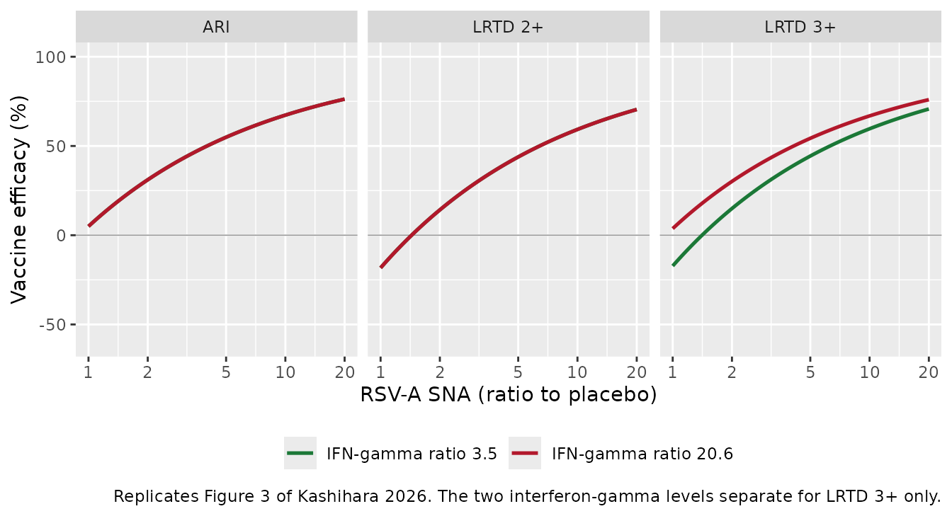
sep <- grid_cmi |>
  group_by(SNA_RSVA_PBORATIO) |>
  summarise(
    d_ari   = diff(range(ve_ari)),
    d_lrtd2 = diff(range(ve_lrtd2)),
    d_lrtd3 = diff(range(ve_lrtd3)),
    .groups = "drop"
  )

stopifnot(
  # No interferon-gamma term on ARI or LRTD 2+: the two curves must be
  # IDENTICAL, not merely close.
  max(sep$d_ari)   < 1e-10,
  max(sep$d_lrtd3) > 0,           # ... and LRTD 3+ must actually separate
  max(sep$d_lrtd2) < 1e-10,
  # Higher cell-mediated immunity gives higher efficacy: the paper's
  # conclusion that "CMI may be correlated with additional clinical benefits
  # in mitigating the severity of RSV infection".
  all(grid_cmi$ve_lrtd3[grid_cmi$IFNG_PBORATIO == 20.6] >
      grid_cmi$ve_lrtd3[grid_cmi$IFNG_PBORATIO == 3.5])
)

sep |>
  filter(SNA_RSVA_PBORATIO %in% range(SNA_RSVA_PBORATIO)) |>
  mutate(across(starts_with("d_"), \(x) round(x, 2))) |>
  dplyr::rename("RSV-A SNA ratio" = SNA_RSVA_PBORATIO,
                "ARI spread (%)" = d_ari,
                "LRTD 2+ spread (%)" = d_lrtd2,
                "LRTD 3+ spread (%)" = d_lrtd3) |>
  knitr::kable(digits = 2, caption = paste(
    "Spread in predicted VE between interferon-gamma ratios 3.5 and 20.6.",
    "Zero for ARI and LRTD 2+ by construction; positive for LRTD 3+."
))| RSV-A SNA ratio | ARI spread (%) | LRTD 2+ spread (%) | LRTD 3+ spread (%) |
|---|---|---|---|
| 1 | 0 | 0 | 20.94 |
| 20 | 0 | 0 | 5.23 |
Why the common SNA slope is smaller than the primary LRTD 3+ slope
The paper reconciles its two models explicitly:
“The common SNA effect in MI (0.321, SE = 0.091) was comparable to the SNA effect on RSV-ARI (0.323, SE = 0.110) and RSV-LRTD2+ (0.285, SE = 0.110) in the primary SNA-VE analysis but smaller than the SNA effect on RSV-LRTD3+ (0.517, SE = 0.117) estimated in the primary analysis. The smaller effect could be explained by part of the contribution to VE for RSV-LRTD3+ being accounted for by the IFN-gamma effect.” (Results 3.3)
get_theta <- function(model, nm) {
  th <- rxode2::rxode(model)$theta
  v  <- th[[nm]]
  if (length(v) != 1L || is.na(v)) stop("no unique theta '", nm, "'")
  v
}

slopes <- tibble::tibble(
  quantity = c("Primary: SNA slope on ARI",
               "Primary: SNA slope on LRTD 2+",
               "Primary: SNA slope on LRTD 3+",
               "Secondary: common SNA slope",
               "Secondary: IFN-gamma slope on LRTD 3+"),
  value = c(get_theta(mod_sna,    "e_sna_tve_ari"),
            get_theta(mod_sna,    "e_sna_tve_lrtd2"),
            get_theta(mod_sna,    "e_sna_tve_lrtd3"),
            get_theta(mod_snacmi, "e_sna_tve"),
            get_theta(mod_snacmi, "e_ifng_tve_lrtd3"))
)
#> ℹ parameter labels from comments will be replaced by 'label()'
#> ℹ parameter labels from comments will be replaced by 'label()'
#> ℹ parameter labels from comments will be replaced by 'label()'
#> ℹ parameter labels from comments will be replaced by 'label()'
#> ℹ parameter labels from comments will be replaced by 'label()'

common <- get_theta(mod_snacmi, "e_sna_tve")
#> ℹ parameter labels from comments will be replaced by 'label()'
stopifnot(
  # "comparable to" ARI and LRTD 2+ ...
  abs(common - get_theta(mod_sna, "e_sna_tve_ari"))   < 0.05,
  abs(common - get_theta(mod_sna, "e_sna_tve_lrtd2")) < 0.05,
  # ... "but smaller than" the primary LRTD 3+ slope, by a clear margin.
  get_theta(mod_sna, "e_sna_tve_lrtd3") - common > 0.15
)
#> ℹ parameter labels from comments will be replaced by 'label()'
#> ℹ parameter labels from comments will be replaced by 'label()'
#> ℹ parameter labels from comments will be replaced by 'label()'

slopes |>
  dplyr::rename("Quantity" = quantity, "Estimate" = value) |>
  knitr::kable(digits = 3, caption = paste(
    "Slope estimates read back from the packaged models, reproducing the",
    "comparison in Kashihara 2026 Results 3.3."
))| Quantity | Estimate |
|---|---|
| Primary: SNA slope on ARI | 0.323 |
| Primary: SNA slope on LRTD 2+ | 0.285 |
| Primary: SNA slope on LRTD 3+ | 0.517 |
| Secondary: common SNA slope | 0.321 |
| Secondary: IFN-gamma slope on LRTD 3+ | 0.111 |
Assumptions and deviations
No PKNCA validation. This is a study-level meta-regression with no concentrations, no dosing and no time course, so NCA is not a meaningful check. It is replaced above by structural checks on the analysis dataset, exact replication of the paper’s two published numeric predictions, a between-trial variability recovery check, and replication of Figures 1 and 3.
Residual error is not published, so it is a placeholder. Kashihara 2026 Equation 1 defines a residual
eps_ikthat was “weighted by the SE of VE at clinical severity level k in the active arm j of study i”, fitted innlme. Neither the residual scale parameter nor the per-observation weights appear anywhere in the paper or Table 3. Rather than invent a variance, each output carriesaddSd_ve_* <- fixed(0.001), which exists only so rxode2 has an error model to attach to the typical-value prediction. It is not a published quantity and must not be read as one. The between-trial variability (eta_study_tve) is published and is encoded from the reported SD.The residual is additive on the transformed scale, but the placeholder is attached to the percent scale. The paper’s
eps_ikis additive on-log(1 - VE/100); the model files declare their endpoints on the back-transformed percent scale because that is the scale the paper tabulates (Table 2) and plots (Figures 1-3), and because the placeholder carries no published information either way. The between-trial eta is applied on the transformed scale, exactly as Equation 1 specifies.Sensitivity analyses are not extracted. Table 3’s
RSV-B SNA / Sensitivity analysis based on MI approachcolumns are a subtype-swap robustness check, and the leave-one-out analysis (Figure S13) is a stability check. Per the library’s replicate-the-author’s-structure policy, robustness analyses that the authors did not report as a final model are excluded. The paper found the RSV-B results “comparable” to RSV-A, consistent with the Spearman correlation of 0.89 between the two subtypes’ SNA.The secondary model encodes the MI estimates, not the CCA estimates. Kashihara 2026 Results 3.3 describes the complete-case fit as the development step and multiple imputation as the extension to the full dataset “without altering the model structure”; Figure 3, the published simulation of this model, is “based on the MI model”, with the CCA simulation relegated to Figure S9. The CCA values are recorded in the source trace table above for reference.
The interferon-gamma confidence interval is much wider than its standard error implies. Table 3 reports
IFN-g slope on RSV-LRTD3+as 0.111 with SE 0.138 but a 95% CI of [-2.00, 2.23]. This is not a transcription error: the interval is a Rubin’s-rules interval on a t-distribution whose degrees of freedom collapse when the fraction of missing information is large, and only four of seven trials had an observed interferon-gamma value. The point estimate is what the model encodes. The paper is explicit that this analysis is exploratory and that “no definitive conclusions can be drawn regarding the contribution of CMI to VE”; the extracted model should be used in that spirit.Two new canonical covariate columns were registered for this extraction:
SNA_RSVA_PBORATIOandIFNG_PBORATIO, forming a<ANALYTE>_RATIOfamily of placebo-corrected, study-arm-level vaccine immunogenicity readouts. Both are documented ininst/references/covariate-columns.md.IFNG_PBORATIOis deliberately not an alias of the existingIFNGcanonical, which is an absolute serum concentration in pg/mL used for target-mediated-disposition scaling; the two differ in units, level of aggregation, and meaning.Trial-level, not subject-level. Both models simulate the efficacy a trial would report given its arm-level immunogenicity. They cannot simulate an individual participant’s outcome, and
eta_study_tvemust not be reinterpreted as between-subject variability.Extrapolation limits. The calibrated range is an RSV-A SNA ratio of roughly 1.5 to 14 and an interferon-gamma ratio of roughly 3.5 to 20.6. The paper notes that the data lack “a moderate SNA ratio of 3 to 7”, and suggests a sigmoid Emax relationship might describe LRTD 2+ better but could not be fitted for want of data in that gap. Predictions in and beyond that gap should be treated accordingly.
The observed-vs-predicted overlay uses the paper’s tabulated values. Original participant-level data are not public. Figure 1’s overlaid points are Kashihara 2026 Table 2 verbatim, not a digitisation of the published figure.