Denosumab MB09 biosimilar (Sanchez-Vidaurre 2025)
Source:vignettes/articles/SanchezVidaurre_2025_denosumab.Rmd
SanchezVidaurre_2025_denosumab.RmdModel and source
- Citation: Sanchez-Vidaurre S, Paravisini A, Queiruga-Parada J. Population PK Modeling of Denosumab Biosimilar MB09 and Reference Denosumab to Establish PK Similarity. Pharmaceutics. 2025;17(9):1146. doi:10.3390/pharmaceutics17091146
- Article (open access): https://doi.org/10.3390/pharmaceutics17091146
- Supplement (Figure S1, Tables S1-S3): https://www.mdpi.com/article/10.3390/pharmaceutics17091146/s1
Sanchez-Vidaurre 2025 is a population PK meta-analysis supporting the biosimilarity of MB09 (mAbxience) to the denosumab reference products Xgeva and Prolia. The authors fitted the same structure twice:
-
SanchezVidaurre_2025_denosumab_phase1- the fit to the phase I study alone (Table 3; the estimates quoted in the abstract), which the model-based bioequivalence assessment at 35 mg rests on. -
SanchezVidaurre_2025_denosumab- the final model fitted to the phase I and phase III studies pooled (Table 4), with a study effect on V/F. The paper uses it for the 60 mg and 120 mg simulations (Figures 3 and 4).
Both are one-compartment models with first-order subcutaneous absorption and parallel linear and Michaelis-Menten elimination, body weight on linear clearance as a power term centred on 70 kg, log-normal inter-individual variability on KA, V/F and CL/F, and a proportional residual error.
#> ℹ parameter labels from comments will be replaced by 'label()'- SanchezVidaurre_2025_denosumab_phase1 - One-compartment population PK model with first-order subcutaneous absorption and parallel linear and Michaelis-Menten elimination for denosumab (MB09 biosimilar and EU- and US-sourced Xgeva, pooled) after a single 35 mg subcutaneous dose in healthy adult men (phase I study MB09-A-01-19). Body weight enters linear clearance as a power term centred on 70 kg; log-normal inter-individual variability on ka, V/F and CL/F; proportional residual error. This is the phase-I-only fit of Sanchez-Vidaurre 2025 (Table 3, the abstract’s headline estimates) used for the model-based bioequivalence assessment; the companion pooled phase I + phase III final model is SanchezVidaurre_2025_denosumab.
#> ℹ parameter labels from comments will be replaced by 'label()'- SanchezVidaurre_2025_denosumab - One-compartment population PK model with first-order subcutaneous absorption and parallel linear and Michaelis-Menten elimination for denosumab (MB09 biosimilar and reference Xgeva / Prolia, pooled), fitted to a phase I study in healthy adult men (single 35 mg SC dose) and a phase III study in postmenopausal women with osteoporosis (60 mg SC every 6 months). Body weight enters linear clearance as a power term centred on 70 kg and study enters V/F; log-normal inter-individual variability on ka, V/F and CL/F; proportional residual error. Final model of Sanchez-Vidaurre 2025 (Table 4). The study effect on V/F (-0.534) is encoded as printed with the phase I study as reference, but the paper does not state its form or coding and this reading does not reproduce the paper’s own phase III figures; see the vignette before using STUDY_MB09C0119 = 1. The phase-I-only fit is SanchezVidaurre_2025_denosumab_phase1.
Read before simulating phase III women with the final
model. Table 4 prints the study effect on V/F as
Study~V = -0.534 without its functional form, its coding or
its reference study. The model encodes it as
V/F = 9.00 * exp(-0.534 * STUDY_MB09C0119), with the phase
I study as the reference, so phase III women get V/F = 5.27 L. That
reading over-predicts the paper’s own phase III simulation (Figure 3) by
about 1.7-fold at the peak, and the opposite coding contradicts the
phase I results. The section Study effect
on V/F below shows the comparison.
Population
Sanchez-Vidaurre 2025 Tables 1 and 2 and Results 3.1:
- Phase I, MB09-A-01-19 (NCT05299073). 255 healthy White men (85 per arm) given a single 35 mg SC dose of MB09, EU-sourced Xgeva or US-sourced Xgeva; mean age 39.5 years (SD 6.90), weight 82.97 kg (SD 8.49), height 178.7 cm. Rich sampling from pre-dose to day 253; 4,256 samples.
- Phase III, MB09-C-01-19 (SIMBA, NCT05338086). 555 postmenopausal women with osteoporosis (278 MB09, 277 EU-Prolia) given 60 mg SC every 6 months; mean age 65.8 years (SD 5.94), weight 63.20 kg (SD 8.79); 99.3% White. Sparse sampling at day 1 (pre-dose), day 11 and months 1, 3, 6 and 12; 3,026 samples.
Serum denosumab was measured with a validated Meso Scale Discovery
electrochemiluminescence assay. Models were fitted in NONMEM 7.4.3
(ADVAN13, FOCE with interaction). Treatment (MB09 vs reference) was
tested on every PK parameter and was not retained (Results 3.2.2), so
all products share the same parameters; the model files record this in
covariatesDataExcluded.
Source trace
| Equation / parameter | Phase I model (Table 3) | Final model (Table 4) | Source location |
|---|---|---|---|
| Structure: 1-cmt, first-order SC absorption, linear + Michaelis-Menten elimination | yes | yes | Methods 2.3.1; Results 3.2.1, 3.2.3 |
lka (KA, 1/day) |
0.406 | 0.349 | Tables 3 / 4, row ‘KA’ |
lvc (V/F, L) |
9.33 | 9.00 | Tables 3 / 4, row ‘V/F’ |
lcl (CL/F at 70 kg, L/day) |
0.123 | 0.143 | Tables 3 / 4, row ‘CL/F’ |
e_wt_cl (exponent on WT/70) |
1.32 | 1.07 | Tables 3 / 4, row ‘BW~CL’; centring at 70 kg from Methods 2.3.3 |
lkm (Km, ug/mL) |
0.124 | 0.162 | Tables 3 / 4, row ‘Km (ng/mL)’; unit corrected, see Assumptions |
lvmax (Vm, mg/day) |
0.139 | 0.128 | Tables 3 / 4, row ‘Vm (ng/day)’; unit corrected, see Assumptions |
e_study_mb09c0119_vc |
- | -0.534 | Table 4, row ‘Study~V’; form and coding unprinted |
etalka (CV) |
61% | 60% | Tables 3 / 4, IIV column |
etalvc (CV) |
13% | 15.7% | Tables 3 / 4, IIV column |
etalcl (CV) |
37% | 34.6% | Tables 3 / 4, IIV column |
propSd |
0.17 | 0.195 | Tables 3 / 4, row ‘Residual variability’; proportional model, Results 3.2.1 |
IIV form P = exp(MU + ETA)
|
yes | yes | Methods 2.3.2, Eqs 1-2 |
Shared simulation helpers
set.seed(20251146) # weights (base R)
rxode2::rxSetSeed(20251146) # random effects and residuals (rxode2)

mod_p1 <- readModelDb("SanchezVidaurre_2025_denosumab_phase1")
mod_fin <- readModelDb("SanchezVidaurre_2025_denosumab")

# Weight distributions from Table 2 (mean, SD), truncated at +/- 2.5 SD.
draw_wt <- function(n, mean, sd) {
  pmin(pmax(rnorm(n, mean, sd), mean - 2.5 * sd), mean + 2.5 * sd)
}

# One SC dose at time 0 plus observation rows on the central compartment.
make_events <- function(cohort, dose, obs_times) {
  dose_rows <- cohort |>
    mutate(time = 0, amt = dose, evid = 1L, cmt = "depot")
  obs_rows <- cohort |>
    tidyr::crossing(time = obs_times) |>
    mutate(amt = 0, evid = 0L, cmt = "central")
  bind_rows(dose_rows, obs_rows) |>
    arrange(id, time, desc(evid)) |>
    as.data.frame()
}

sim_cohort <- function(mod, events, keep_cols, ...) {
  sim <- rxode2::rxSolve(mod, events, returnType = "data.frame", ...)
  sim |>
    select(id, time, Cc) |>
    left_join(distinct(events[, c("id", keep_cols)]), by = "id") |>
    # ug/mL -> ng/mL, the paper's unit. Once the Michaelis-Menten arm empties
    # the central compartment the solver returns values of order -1e-9 ng/mL;
    # they are numerical noise and are set to zero.
    mutate(conc = pmax(Cc, 0) * 1000)
}

obs_grid <- sort(unique(c(0, 1 / 3, 2 / 3, 1, 2, 3, 5, 7, 10, 14, 21, seq(28, 546, by = 7))))
Phase I model: 35 mg in healthy men
Typical-value check against Supplementary Table 2
Supplementary Table 2 summarises the model-based Cmax and AUC for each phase I arm (N = 85 each). A typical subject at the phase I mean weight (83 kg) should sit inside the range of the three arms’ geometric means.
typ_ev <- make_events(
  data.frame(id = 1L, WT = 82.97, STUDY_MB09C0119 = 0L),
  dose = 35, obs_times = seq(0, 400, by = 0.05)
)
typ_p1 <- rxode2::rxSolve(rxode2::zeroRe(mod_p1), typ_ev, returnType = "data.frame")
#> ℹ parameter labels from comments will be replaced by 'label()'
#> ℹ omega/sigma items treated as zero: 'etalka', 'etalvc', 'etalcl'
typ_p1_nca <- c(
  cmax = max(typ_p1$Cc) * 1000,
  aucinf = sum(diff(typ_p1$time) * (head(typ_p1$Cc, -1) + tail(typ_p1$Cc, -1)) / 2) * 1000
)
typ_p1_nca
#>       cmax     aucinf
#>   3171.688 141637.565

stopifnot(
  # Supplementary Table 2 Cmax geometric means 3,020-3,188 ng/mL
  typ_p1_nca[["cmax"]] > 0.95 * 3020, typ_p1_nca[["cmax"]] < 1.05 * 3188,
  # Supplementary Table 2 AUCinf geometric means 136,115-148,433 day*ng/mL
  typ_p1_nca[["aucinf"]] > 0.95 * 136115, typ_p1_nca[["aucinf"]] < 1.05 * 148433
)
The typical profile has fallen to a negligible concentration well before day 400, so the trapezoidal sum on the 0.05-day grid is the full AUC0-inf of this deterministic solve.
Virtual cohort and Figure 2
cohort_p1 <- data.frame(
  id = 1:255,
  treatment = rep(c("MB09", "EU-Xgeva", "US-Xgeva"), each = 85),
  WT = draw_wt(255, 82.97, 8.492),
  STUDY_MB09C0119 = 0L
)
ev_p1 <- make_events(cohort_p1, dose = 35, obs_times = obs_grid)
sim_p1 <- sim_cohort(mod_p1, ev_p1, keep_cols = c("treatment", "WT"))
#> ℹ parameter labels from comments will be replaced by 'label()'
fig2_digitised <- bind_rows(
  data.frame(
    source = "Figure 2 simulated median",
    time = c(10, 28, 56, 84, 98, 112),
    conc = c(2900, 2200, 1000, 380, 180, 65)
  ),
  data.frame(
    source = "Figure 2 observed median",
    time = c(10, 28, 56, 84, 98, 112, 140),
    conc = c(3000, 2300, 1050, 400, 190, 110, 43)
  )
)

pct_p1 <- sim_p1 |>
  filter(time > 0) |>
  group_by(time) |>
  summarise(
    p05 = quantile(conc, 0.05), p50 = median(conc), p95 = quantile(conc, 0.95),
    .groups = "drop"
  ) |>
  # Cleared profiles are exactly zero; floor them below the plotted range so
  # the log axis can draw them.
  mutate(across(c(p05, p50, p95), \(x) pmax(x, 1)))

ggplot(pct_p1, aes(time)) +
  geom_ribbon(aes(ymin = p05, ymax = p95), fill = "tomato", alpha = 0.15) +
  geom_line(aes(y = p50), colour = "tomato", linewidth = 1) +
  geom_point(
    data = fig2_digitised, aes(y = conc, shape = source), size = 2.5
  ) +
  scale_shape_manual(values = c(16, 1)) +
  scale_y_log10() +
  coord_cartesian(xlim = c(0, 160), ylim = c(10, 10000)) +
  labs(x = "Time (days)", y = "Denosumab (ng/mL)", shape = NULL) +
  theme_bw() +
  theme(legend.position = "bottom")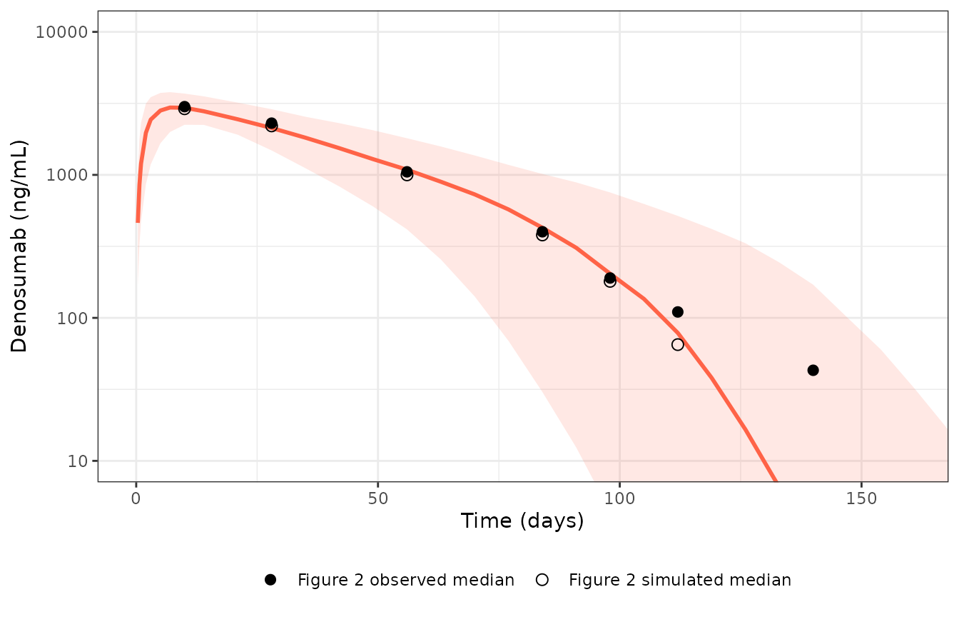
Replicates Figure 2 of Sanchez-Vidaurre 2025: 35 mg single SC dose in healthy men, phase I model. Red: 5th, 50th and 95th percentiles of the simulated cohort. Points: simulated (open) and observed (filled) medians digitised by the maintainers from Figure 2.
PKNCA against Supplementary Table 2
The simulation grid runs to day 546. The Michaelis-Menten arm clears the last of the drug quickly once concentrations fall below Km, so every simulated profile is effectively zero well before then and AUC0-last is AUC0-inf; the check below confirms the AUC still accruing over the last eight weeks is negligible. Supplementary Table 2 reports AUC0-inf medians, and its AUC0-6 months differs from them by less than 0.3%.
conc_p1 <- sim_p1 |> filter(!is.na(Cc))
dose_p1 <- cohort_p1 |> mutate(time = 0, amt = 35)

nca_p1 <- PKNCA::pk.nca(PKNCA::PKNCAdata(
  PKNCA::PKNCAconc(conc_p1, conc ~ time | treatment + id),
  PKNCA::PKNCAdose(dose_p1, amt ~ time | treatment + id),
  intervals = data.frame(
    start = 0, end = Inf, cmax = TRUE, tmax = TRUE, auclast = TRUE
  )
))

nca_p1_wide <- as.data.frame(nca_p1$result) |>
  filter(PPTESTCD %in% c("cmax", "auclast")) |>
  select(treatment, id, PPTESTCD, PPORRES) |>
  tidyr::pivot_wider(names_from = PPTESTCD, values_from = PPORRES)

# Supplementary Table 2 medians (model-based individual predictions, N = 85 per arm).
published_p1 <- data.frame(
  treatment = c("MB09", "EU-Xgeva", "US-Xgeva"),
  cmax = c(3243, 3095, 3156),
  auclast = c(150861, 139353, 139245)
)

cmp_p1 <- nlmixr2lib::ncaComparisonTable(
  simulated = nca_p1_wide |> select(treatment, cmax, auclast),
  reference = published_p1,
  by = "treatment",
  units = c(cmax = "ng/mL", auclast = "day*ng/mL"),
  tolerance_pct = 20
)
knitr::kable(
  cmp_p1,
  caption = paste(
    "Phase I model, 35 mg: simulated medians vs Supplementary Table 2 medians.",
    "* differs from reference by >20%."
  )
)| NCA parameter | treatment | Reference | Simulated | % diff |
|---|---|---|---|---|
| Cmax (ng/mL) | MB09 | 3240 | 3000 | -7.4% |
| Cmax (ng/mL) | EU-Xgeva | 3100 | 3110 | +0.4% |
| Cmax (ng/mL) | US-Xgeva | 3160 | 3080 | -2.4% |
| AUClast (day*ng/mL) | MB09 | 151000 | 143000 | -5.4% |
| AUClast (day*ng/mL) | EU-Xgeva | 139000 | 139000 | -0.2% |
| AUClast (day*ng/mL) | US-Xgeva | 139000 | 145000 | +4.3% |
# AUC accrued after day 490 as a fraction of the total (90th percentile of subjects).
tail_frac <- sim_p1 |>
  group_by(id) |>
  summarise(
    frac = sum(diff(time[time >= 490]) * head(conc[time >= 490], -1)) /
      sum(diff(time) * head(conc, -1)),
    .groups = "drop"
  )
stopifnot(quantile(tail_frac$frac, 0.9) < 1e-3)
pooled_p1 <- nca_p1_wide |>
  summarise(cmax = median(cmax), aucinf = median(auclast))
pct_cmax_p1 <- 100 * (pooled_p1$cmax / median(published_p1$cmax) - 1)
pct_auc_p1 <- 100 * (pooled_p1$aucinf / median(published_p1$auclast) - 1)
c(cmax_pct = pct_cmax_p1, aucinf_pct = pct_auc_p1)
#>   cmax_pct aucinf_pct
#>  -2.404788   2.647174
stopifnot(abs(pct_cmax_p1) < 15, abs(pct_auc_p1) < 15)
The three arms share one set of parameters (treatment was not a covariate), so per-arm differences in the simulated column are sampling noise; the paper’s MB09 arm happens to sit about 8% above the two Xgeva arms.
Final model
Study effect on V/F
The final model is simulated two ways for a single 60 mg dose in 200
phase III women (Table 2 weights): with the study term as encoded
(STUDY_MB09C0119 = 1, V/F 5.27 L) and with the study term
switched off (STUDY_MB09C0119 = 0, V/F 9.00 L). Figure 3 of
the paper is the final-model simulation for this cohort.
cohort_p3 <- data.frame(id = 1:200, WT = draw_wt(200, 63.196, 8.787))
cohort_fig3 <- bind_rows(
  cohort_p3 |> mutate(scenario = "Study term as encoded (STUDY_MB09C0119 = 1)", STUDY_MB09C0119 = 1L),
  cohort_p3 |> mutate(scenario = "Study term off (STUDY_MB09C0119 = 0)", STUDY_MB09C0119 = 0L, id = id + 200L)
)
ev_fig3 <- make_events(cohort_fig3, dose = 60, obs_times = obs_grid[obs_grid <= 210])
sim_fig3 <- sim_cohort(mod_fin, ev_fig3, keep_cols = c("scenario", "WT"))
#> ℹ parameter labels from comments will be replaced by 'label()'
fig3_digitised <- bind_rows(
  data.frame(
    source = "Figure 3 simulated median",
    time = c(10, 36, 90, 112, 140, 168),
    conc = c(5100, 3300, 800, 400, 100, 14)
  ),
  data.frame(
    source = "Figure 3 observed median",
    time = c(11, 36, 90, 182),
    conc = c(6000, 4300, 1200, 100)
  )
)

pct_fig3 <- sim_fig3 |>
  filter(time > 0) |>
  group_by(scenario, time) |>
  summarise(
    p05 = quantile(conc, 0.05), p50 = median(conc), p95 = quantile(conc, 0.95),
    .groups = "drop"
  ) |>
  # Cleared profiles are exactly zero; floor them below the plotted range so
  # the log axis can draw them.
  mutate(across(c(p05, p50, p95), \(x) pmax(x, 1)))

ggplot(pct_fig3, aes(time)) +
  geom_ribbon(aes(ymin = p05, ymax = p95, fill = scenario), alpha = 0.12) +
  geom_line(aes(y = p50, colour = scenario), linewidth = 1) +
  geom_point(data = fig3_digitised, aes(y = conc, shape = source), size = 2.5) +
  scale_shape_manual(values = c(16, 1)) +
  scale_y_log10() +
  coord_cartesian(xlim = c(0, 210), ylim = c(10, 20000)) +
  labs(x = "Time (days)", y = "Denosumab (ng/mL)", colour = NULL, fill = NULL, shape = NULL) +
  theme_bw() +
  theme(legend.position = "bottom", legend.direction = "vertical")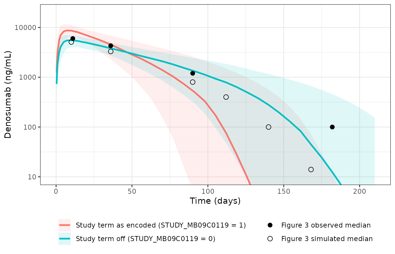
Replicates Figure 3 of Sanchez-Vidaurre 2025: 60 mg single SC dose in postmenopausal women, final model. Lines and bands: simulated median and 5th-95th percentiles for each reading of the study term. Points: simulated (open) and observed (filled) medians digitised by the maintainers from Figure 3.
fig3_check <- pct_fig3 |>
  filter(time %in% c(10, 35, 91)) |>
  select(scenario, time, p50) |>
  tidyr::pivot_wider(names_from = time, values_from = p50, names_prefix = "day_")
fig3_check |>
  dplyr::rename(
    "Scenario" = scenario,
    "Median day 10 (ng/mL)" = day_10,
    "Median day 35 (ng/mL)" = day_35,
    "Median day 91 (ng/mL)" = day_91
  ) |>
  knitr::kable(
    digits = 0,
    caption = "Simulated median vs Figure 3 (simulated median about 5,100 at day 10, 3,300 at day 36, 800 at day 90)."
)| Scenario | Median day 10 (ng/mL) | Median day 35 (ng/mL) | Median day 91 (ng/mL) |
|---|---|---|---|
| Study term as encoded (STUDY_MB09C0119 = 1) | 8633 | 4691 | 510 |
| Study term off (STUDY_MB09C0119 = 0) | 5543 | 3877 | 1330 |
peak <- pct_fig3 |>
  group_by(scenario) |>
  summarise(peak = max(p50), .groups = "drop")
peak_on <- peak$peak[grepl("= 1", peak$scenario)]
peak_off <- peak$peak[grepl("= 0", peak$scenario)]
c(peak_encoded = peak_on, peak_off = peak_off, figure3 = 5100)
#> peak_encoded     peak_off      figure3
#>     8718.392     5542.820     5100.000
# The encoded study term moves the phase III peak well away from Figure 3; the
# reading without it lands close. This documents the conflict described above.
stopifnot(
  abs(log(peak_off / 5100)) < abs(log(peak_on / 5100)),
  peak_on / 5100 > 1.3
)
With the study term as encoded the simulated phase III median peaks
near 8700 ng/mL against about 5,100 ng/mL in Figure 3; with it switched
off the peak is 5500 ng/mL. Applying the term to the phase I men instead
(exp(-0.534) on the phase I V/F) would push their 35 mg
peak to about 5,000 ng/mL against the 3,000-3,200 ng/mL of Supplementary
Table 2 and Figure 2. No coding of the printed coefficient reproduces
both studies, which is why the term is flagged.
Neither reading reproduces the whole of Figure 3. The published simulated median peaks like the reading without the term, but its terminal phase falls between the two: about 800 ng/mL at day 90, against 510 ng/mL with the term and 1330 ng/mL without it at day 91. The published figure may also differ in its virtual cohort, which the paper does not describe beyond the study.
120 mg (Figure 4 and Results 3.5)
Figure 4 and the mean AUC0-inf in Results 3.5 come from a single 120 mg dose given to virtual subjects carrying the covariates of all 810 study subjects. Here 200 subjects keep the 255:555 proportion (63 men with phase I weights, 137 women with phase III weights).
cohort_120 <- bind_rows(
  data.frame(id = 1:63, WT = draw_wt(63, 82.97, 8.492), STUDY_MB09C0119 = 0L),
  data.frame(id = 64:200, WT = draw_wt(137, 63.196, 8.787), STUDY_MB09C0119 = 1L)
)
cohort_fig4 <- bind_rows(
  cohort_120 |> mutate(scenario = "Study term as encoded"),
  cohort_120 |> mutate(scenario = "Study term off", STUDY_MB09C0119 = 0L, id = id + 200L)
)
ev_fig4 <- make_events(cohort_fig4, dose = 120, obs_times = obs_grid)
sim_fig4 <- sim_cohort(mod_fin, ev_fig4, keep_cols = c("scenario", "WT"))
fig4_digitised <- data.frame(
  time = c(8, 25, 50, 75, 100, 125, 150, 168),
  conc = c(10500, 9000, 5000, 2700, 1400, 650, 300, 150)
)
pct_fig4 <- sim_fig4 |>
  filter(time > 0) |>
  group_by(scenario, time) |>
  summarise(
    p05 = quantile(conc, 0.05), p50 = median(conc), p95 = quantile(conc, 0.95),
    .groups = "drop"
  ) |>
  # Cleared profiles are exactly zero; floor them below the plotted range so
  # the log axis can draw them.
  mutate(across(c(p05, p50, p95), \(x) pmax(x, 1)))
ggplot(pct_fig4, aes(time)) +
  geom_ribbon(aes(ymin = p05, ymax = p95, fill = scenario), alpha = 0.12) +
  geom_line(aes(y = p50, colour = scenario), linewidth = 1) +
  geom_point(data = fig4_digitised, aes(y = conc), size = 2.5) +
  scale_y_log10() +
  coord_cartesian(xlim = c(0, 260), ylim = c(10, 30000)) +
  labs(x = "Time (days)", y = "Denosumab (ng/mL)", colour = NULL, fill = NULL) +
  theme_bw() +
  theme(legend.position = "bottom")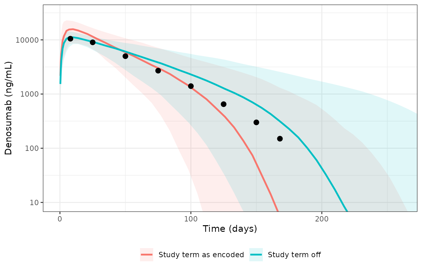
Replicates Figure 4 of Sanchez-Vidaurre 2025: 120 mg single SC dose, final model. Lines and bands: simulated median and 5th-95th percentiles. Points: median digitised by the maintainers from Figure 4.
conc_120 <- sim_fig4 |> filter(!is.na(Cc))
dose_120 <- cohort_fig4 |> mutate(time = 0, amt = 120)
nca_120 <- PKNCA::pk.nca(PKNCA::PKNCAdata(
  PKNCA::PKNCAconc(conc_120, conc ~ time | scenario + id),
  PKNCA::PKNCAdose(dose_120, amt ~ time | scenario + id),
  intervals = data.frame(start = 0, end = Inf, cmax = TRUE, auclast = TRUE)
))
auc_120 <- as.data.frame(nca_120$result) |>
  filter(PPTESTCD == "auclast") |>
  group_by(scenario) |>
  summarise(mean_auc = mean(PPORRES), sd_auc = sd(PPORRES), .groups = "drop") |>
  mutate(pct_diff_mean = 100 * (mean_auc / 753000 - 1))
auc_120 |>
  dplyr::rename(
    "Scenario" = scenario,
    "Mean AUC0-inf (day*ng/mL)" = mean_auc,
    "SD" = sd_auc,
    "Mean vs 753,000 (%)" = pct_diff_mean
  ) |>
  knitr::kable(
    digits = 0,
    caption = "Mean AUC0-inf after 120 mg vs Results 3.5 (753,000, SD 285,200 day*ng/mL)."
)| Scenario | Mean AUC0-inf (day*ng/mL) | SD | Mean vs 753,000 (%) |
|---|---|---|---|
| Study term as encoded | 780169 | 305086 | 4 |
| Study term off | 756628 | 266232 | 0 |
The pattern of Figure 3 repeats here: the published median peaks with the reading without the term and declines between the two readings. The 120 mg mean AUC cannot separate them: both are within a few percent of the published 753,000, because at this dose most of the drug is cleared by the linear arm, whose share of the AUC (dose / CL) does not depend on V/F. (Results 3.5 gives no unit; the value is on the dayng/mL scale of Supplementary Table 2. The Discussion’s comparison value of 723,000 is labelled ngh/mL, which on that scale would be about 24-fold too small, so that label is taken to be a slip.)
Assumptions and deviations
- Km and Vm units. Tables 3 and 4 print Km in ng/mL and Vm in ng/day. Read literally, the Michaelis-Menten arm is either negligible (Km 0.124 ng/mL is below any concentration in the data) or, with Vm in mg/day, a constant 0.139 mg/day sink that drives the 35 mg profile below zero. Read as Km in ug/mL (= mg/L, with amounts in mg and V/F in L) and Vm in mg/day, the phase I model reproduces Supplementary Table 2 (typical-value check above), whereas the linear arm alone would give an AUC0-inf of about 227,000 day*ng/mL. Both models carry the corrected units. The abstract repeats the printed units.
-
Study effect on V/F (final model). The coefficient
-0.534 is encoded as
exp(-0.534 * STUDY_MB09C0119)with the phase I study as the reference, because the paper states all parameters were MU-referenced (Results 3.2.1) and the pooled V/F of 9.00 L sits next to the phase-I-only 9.33 L. The peaks of the paper’s own Figures 3 and 4 are reproduced without the term (their terminal phase lies between the two readings), and coding it the other way contradicts Figure 2 and Supplementary Table 2 (see Study effect on V/F). The form, coding and reference study are not printed, so the term is unverified; for phase III simulations compare both settings of the indicator. - IIV. Reported as percentages for exponential random effects; converted as omega^2 = log(1 + CV^2). No covariances are reported, so the random effects are independent.
- Residual error. Eq 3 is printed in additive form, but the text states a proportional model and reports the magnitude as a percentage, so it is encoded as proportional.
- Treatment. MB09, EU-Xgeva, US-Xgeva and EU-Prolia share one parameter set; treatment was tested and not retained (Results 3.2.2).
- Not extracted. Supplementary Table S1 (phase I refit with five subjects excluded) is a sensitivity analysis; its estimates differ marginally from Table 3 and are not provided as a separate model.
- Virtual cohorts. Weights are normal with the Table 2 mean and SD per study, truncated at 2.5 SD; Table 2 gives no ranges. The 120 mg cohort uses 200 subjects in the 255:555 study proportion rather than all 810 subjects’ covariates.
- Errata. No erratum or correction to the paper was found (literature check 2026-11-10).
- Digitised values. The figure overlays are medians read by the maintainers from Figures 2-4 and are approximate (about +/-10%).