Lorlatinib exposure-response for safety and efficacy (Chen 2021)

Model and source

Chen 2021 reports the exposure-response (E-R) analysis that supported the approved 100 mg once-daily dose of lorlatinib, a third-generation ALK/ROS1 tyrosine kinase inhibitor, in ALK-positive non-small cell lung cancer (NSCLC). The analysis uses individual patient data from the first-in-human phase I/II study B7461001 (NCT01970865) and fits five independent binomial logistic regressions with R’s glm(family = "binomial") – four safety endpoints in the 328-patient safety analysis set, and one efficacy endpoint in the 132-patient subset with baseline CNS metastasis.

• Article: https://doi.org/10.1002/cpt.2228 (PMC9290079)
• Upstream population PK model (source of every exposure metric): https://doi.org/10.1002/psp4.12585, packaged as modellib("Chen_2021_lorlatinib")

Three features shape how this paper is packaged.

There is no PK layer in the E-R models themselves. Each is a static landmark regression: one binary outcome per patient, with exposure entering as a scalar per-subject covariate. The exposure metrics come from the companion lorlatinib population PK publication – “a two-compartment model with time-varying clearance” – not from anything solved inside these files. Consequently the five model files contain no d/dt(), no compartments and no time dimension. Unusually for this model class, that upstream PK model is also in this library, so the validation below can drive the E-R models from a genuinely simulated exposure distribution rather than an invented one.

Covariates are neither centred nor scaled. Chen 2021 fits raw covariate values, so each intercept is an extrapolated anchor (the logit at TCHOL = 0, TE = 0, CMAX = 1 ng/mL, and so on) rather than a reference-patient probability. This is the structural difference from the Fukae_2024_valemetostat_* logistic family, whose intercepts are reference-patient probabilities.

Three of the five endpoints retained no exposure term at all, and that is the paper’s result rather than a reporting gap. Nine candidate lorlatinib exposure metrics were screened in linear and log-transformed form for every endpoint; only two safety endpoints kept one.

endpoints <- tibble::tribble(
  ~model,                                       ~endpoint,                        ~set,       ~exposure,
  "Chen_2021_lorlatinib_hypercholesterolemia",  "Hypercholesterolemia grade >= 3", "safety",   "log(Cmax,event)",
  "Chen_2021_lorlatinib_teae_grade3",           "Any TEAE grade >= 3",             "safety",   "log(Ctrough,ss)",
  "Chen_2021_lorlatinib_weight_gain",           "Weight gain grade >= 2",          "safety",   "none retained",
  "Chen_2021_lorlatinib_hypertriglyceridemia",  "Hypertriglyceridemia grade >= 3", "safety",   "none retained",
  "Chen_2021_lorlatinib_icorr",                 "Intracranial ORR (IC-ORR)",       "efficacy", "none retained"
) |>
  dplyr::mutate(
    output = paste0("prob_", sub("^Chen_2021_lorlatinib_", "", model)),
    n      = c(298L, 328L, 328L, 298L, 132L)
  )

# Resolve each model function to an rxUi exactly once. readModelDb() returns
# the model *function*; rxode2::rxode() evaluates it to a ui that works
# anywhere (see known-vignette-failure-patterns.md pattern 7).
mods <- lapply(stats::setNames(endpoints$model, endpoints$model),
               function(m) rxode2::rxode(readModelDb(m)))

endpoints |>
  dplyr::select(
    Endpoint = endpoint, `Analysis set` = set, N = n,
    `Exposure term` = exposure, `Model file` = model
  ) |>
  knitr::kable(caption = "The five models packaged from Chen 2021.")

The five models packaged from Chen 2021.

Endpoint	Analysis set	N	Exposure term	Model file
Hypercholesterolemia grade >= 3	safety	298	log(Cmax,event)	Chen_2021_lorlatinib_hypercholesterolemia
Any TEAE grade >= 3	safety	328	log(Ctrough,ss)	Chen_2021_lorlatinib_teae_grade3
Weight gain grade >= 2	safety	328	none retained	Chen_2021_lorlatinib_weight_gain
Hypertriglyceridemia grade >= 3	safety	298	none retained	Chen_2021_lorlatinib_hypertriglyceridemia
Intracranial ORR (IC-ORR)	efficacy	132	none retained	Chen_2021_lorlatinib_icorr

Population

Three analysis sets are in play and must not be conflated (Chen 2021 Tables 1 and 2).

• Safety (N = 328). Every patient who received at least one dose of lorlatinib, across the phase I dose escalation (10-200 mg q.d. or 35-100 mg b.i.d.) and the phase II expansion (100 mg q.d.). Median age 53.0 years (19-85), median weight 66.79 kg (31.80-155.50), 58% female; race White 51% / Asian 34% / Other 4% / Black 2% / missing 9%. Median baseline total cholesterol 193 mg/dL and triglycerides 107.5 mg/dL. Two patients had no PK data and were assigned typical-value exposures. The four safety models were fitted to 328 (TEAE, weight gain) or 298 (the two lipid endpoints, whose paired baseline laboratory covariate is missing in 28-30 patients) of these.
• Efficacy-ORR (N = 197). The subset who had received at least one prior ALK inhibitor, i.e. phase II expansion cohorts 2-5. No model is packaged from this set – see the Errata.
• Efficacy-IC-ORR (N = 132). Those within the efficacy set with baseline CNS metastasis per independent central review. Median age 51.0 years (29-77), median weight 64.25 kg (31.80-124.70), 60% female; 97% had prior ALK-inhibitor treatment and 58% prior CNS radiotherapy. Median baseline alkaline phosphatase 100.5 U/L and amylase 62.0 U/L.

dplyr::bind_rows(
  tibble::as_tibble(
    readModelDb("Chen_2021_lorlatinib_teae_grade3")()$population[
      c("n_subjects", "sex_female_pct", "age_range", "weight_range")]) |>
    dplyr::mutate(`Analysis set` = "Safety", .before = 1),
  tibble::as_tibble(
    readModelDb("Chen_2021_lorlatinib_icorr")()$population[
      c("n_subjects", "sex_female_pct", "age_range", "weight_range")]) |>
    dplyr::mutate(`Analysis set` = "Efficacy-IC-ORR", .before = 1)
) |>
  dplyr::rename(N = n_subjects, `% female` = sex_female_pct,
                Age = age_range, Weight = weight_range) |>
  knitr::kable(caption = "Analysis sets, read from the packaged `population` metadata.")

Analysis sets, read from the packaged population metadata.

Analysis set	N	% female	Age	Weight
Safety	328	58	median 53.00 years, range 19.00-85.00 (Chen 2021 Table 1, safety population)	median 66.79 kg, range 31.80-155.50 (Chen 2021 Table 1, safety population)
Efficacy-IC-ORR	132	60	median 51.00 years, range 29.00-77.00 (Chen 2021 Table 1, Efficacy-IC-ORR population)	median 64.25 kg, range 31.80-124.70 (Chen 2021 Table 1, Efficacy-IC-ORR population)

Source trace

The per-parameter origin is recorded as an in-file comment next to each ini() entry. The table below collects them in one place.

Model element	Source location
Univariate screening form logit(p) = t1 + t2 * exposure	Methods, “Overview of modeling”, Eq. 1
Covariate screening form logit(p) = base model + t3 * covariates	Methods, “Covariates”, Eq. 2
Backward elimination at alpha = 0.01 (dD > chi2(0.99) = 6.63)	Methods, “Final model development”
Definition of the OR column as exp(estimate)	Methods, “Final model development”, last sentence
Hypercholesterolemia grade >= 3: intercept and all three coefficients	Table 3 row block 1, and Eq. 3
TEAE grade >= 3: intercept and all three coefficients	Table 3 row block 2, and Eq. 4
Weight gain grade >= 2: intercept and both coefficients	Table 3 row block 3 (no printed equation)
Hypertriglyceridemia grade >= 3: intercept and all three coefficients	Table 3 row block 4 (no printed equation)
IC-ORR: intercept and both coefficients	Table 4, and Eq. 5
log(Ctrough,ss) is a NATURAL log	Results, “Exposure-safety” (“is natural log transformed”)
TE is measured in DAYS, censored at the whole on-study duration	Table 3 footnote; Methods, “Base model development”
The nine screened exposure metrics	Methods, “Selection of lorlatinib exposure metrics”
Null exposure result for weight gain and hypertriglyceridemia	Results, “Exposure-safety”, final paragraph
Null exposure result for ORR and IC-ORR	Results, “Exposure-efficacy”
Figure 1 fixed covariates (TE = 41 d, BCHOL = 193 mg/dL) and the “below 25%” claim	Results, “Exposure-safety”, and Figure 1 caption
Figure 2 fixed covariates (TE = 38.75 d, BCHOL = 193 mg/dL) and the “approximately 75%” claim	Results, “Exposure-safety”, and Figure 2 caption
Cmax,P1 mean (SD) 687.11 (141.09) ng/mL; Ctrough,P1 114.97 (40.28) ng/mL	Results, “Exposure-efficacy”
Baseline demographics (age, weight, sex, race, ECOG, prior therapy)	Table 1
Baseline laboratory values (cholesterol, triglycerides, ALP, amylase, CrCL, albumin)	Table 2
Software: R >= 3.0, glm(family = "binomial")	Methods, “Overview of modeling”
Exposure metrics derive from a 2-compartment popPK with time-varying CL	Methods, “Assessments and end points”, ref. 14 (= doi:10.1002/psp4.12585)

Every coefficient is reported twice by the paper itself

Chen 2021 states that “the odds ratio (OR) was calculated by exponentiating the parameter estimates”, so each Table 3 / Table 4 row carries the same number in two columns. That redundancy is what makes the transcription auditable – but it is not an exact identity between the two printed columns, because the Estimate column is rounded to three decimals while the OR column was computed from the unrounded estimate. exp(1.659) = 5.254 against a printed OR of 5.256 is therefore the expected behaviour, not a defect.

The right consistency question is an interval one: does some real number b exist with round(b, 3) equal to the printed Estimate and round(exp(b), 3) equal to the printed OR? Naively comparing round(log(printed OR), 3) against the printed Estimate is too crude – it ignores that the OR column is itself rounded, which matters most exactly where the coefficient is large or the OR is small. Check 2 below asks the interval question, and separately imposes a hard gate that the packaged encoding reproduces exp(estimate) to machine precision.

Structural verification: the models reproduce the published tables

These are static regressions with no ODE, no random effects and no residual error, so the packaged encoding can be checked against the source exactly rather than approximately. Two identities must hold for every model.

1. Solved with every covariate at its neutralising value – zero for a linear term, 1 for a log-transformed term – the predicted logit must equal the published intercept.
2. Moving one covariate by exactly one reported unit (or multiplying a log-transformed exposure by e) must change the odds by exactly the published odds ratio for that row.

This audits all 17 published estimates across Tables 3 and 4.

# The neutralising covariate vector: every linear covariate at 0, every
# log-transformed covariate at 1 (so its log is 0). Solved here, the linear
# predictor collapses to the intercept alone.
zero_cov <- list(
  CMAX = 1, CTROUGH = 1, ALP = 1,          # log-transformed terms
  TCHOL = 0, TRIG = 0, WT = 0, AMYL = 0,   # linear terms
  RACE_ASIAN = 0, T_FIRSTDOSE = 0
)

solve_prob <- function(model, output, overrides = list()) {
  ev <- data.frame(id = 1L, time = 0, amt = 0, evid = 0L)
  for (nm in names(zero_cov))  ev[[nm]] <- zero_cov[[nm]]
  for (nm in names(overrides)) ev[[nm]] <- overrides[[nm]]
  as.data.frame(
    rxode2::rxSolve(model, events = ev, returnType = "data.frame")
  )[[output]][1]
}
odds  <- function(p) p / (1 - p)
logit <- function(p) log(p / (1 - p))

Check 1 – every published intercept

published_int <- tibble::tribble(
  ~model,                                       ~intercept,
  "Chen_2021_lorlatinib_hypercholesterolemia",  -18.829,
  "Chen_2021_lorlatinib_teae_grade3",            -7.995,
  "Chen_2021_lorlatinib_weight_gain",            -4.757,
  "Chen_2021_lorlatinib_hypertriglyceridemia",   -5.113,
  "Chen_2021_lorlatinib_icorr",                   3.929
)

int_check <- published_int |>
  dplyr::left_join(endpoints, by = "model") |>
  dplyr::rowwise() |>
  dplyr::mutate(int_sim = logit(solve_prob(mods[[model]], output))) |>
  dplyr::ungroup()

# Algebraic identity between the published table and the encoded ini()
# values, so an exact tolerance is correct here -- there is no simulated
# cohort and no solver noise to admit.
stopifnot(max(abs(int_check$int_sim - int_check$intercept)) < 1e-9)

int_check |>
  dplyr::transmute(
    Endpoint = endpoint,
    `Intercept, published` = intercept,
    `Intercept, simulated` = round(int_sim, 6)
  ) |>
  knitr::kable(caption = "Reproduces the Intercept row of Chen 2021 Table 3 (four safety endpoints) and Table 4 (IC-ORR).")

Reproduces the Intercept row of Chen 2021 Table 3 (four safety endpoints) and Table 4 (IC-ORR).

Endpoint	Intercept, published	Intercept, simulated
Hypercholesterolemia grade >= 3	-18.829	-18.829
Any TEAE grade >= 3	-7.995	-7.995
Weight gain grade >= 2	-4.757	-4.757
Hypertriglyceridemia grade >= 3	-5.113	-5.113
Intracranial ORR (IC-ORR)	3.929	3.929

Check 2 – every published coefficient and odds ratio

For a linear covariate, the odds ratio is the change in odds per one reported unit (1 mg/dL, 1 kg, 1 U/L, 1 day, or the 0 -> 1 step of the Asian-race indicator). For a log-transformed exposure it is the change per e-fold, which the paper spells out for log(Ctrough,ss): “with every unit increase of log(Ctrough ss), there is a 3.214 increase in the OR”.

published_or <- tibble::tribble(
  ~model_suffix,             ~cov,           ~step,  ~est,     ~or_pub,
  "hypercholesterolemia",    "TCHOL",           1,    0.029,    1.029,
  "hypercholesterolemia",    "T_FIRSTDOSE",    24,    0.004,    1.004,   # 24 h = 1 day
  "hypercholesterolemia",    "CMAX",           NA,    1.659,    5.256,   # multiplicative, e-fold
  "teae_grade3",             "TCHOL",           1,    0.012,    1.012,
  "teae_grade3",             "T_FIRSTDOSE",    24,    0.012,    1.012,
  "teae_grade3",             "CTROUGH",        NA,    1.167,    3.214,
  "weight_gain",             "WT",              1,    0.029,    1.030,
  "weight_gain",             "T_FIRSTDOSE",    24,    0.003,    1.003,
  "hypertriglyceridemia",    "RACE_ASIAN",      1,    1.011,    2.749,
  "hypertriglyceridemia",    "T_FIRSTDOSE",    24,    0.003,    1.003,
  "hypertriglyceridemia",    "TRIG",            1,    0.018,    1.018,
  "icorr",                   "ALP",            NA,   -1.015,    0.363,
  "icorr",                   "AMYL",            1,    0.015,    1.015
) |>
  dplyr::mutate(model = paste0("Chen_2021_lorlatinib_", model_suffix))

or_check <- published_or |>
  dplyr::left_join(endpoints, by = "model") |>
  dplyr::rowwise() |>
  dplyr::mutate(
    # A log-transformed covariate (step = NA) moves multiplicatively by e;
    # a linear covariate moves additively by `step`.
    new_val = if (is.na(step)) exp(1) * zero_cov[[cov]] else zero_cov[[cov]] + step,
    p0      = solve_prob(mods[[model]], output),
    p1      = solve_prob(mods[[model]], output,
                         stats::setNames(list(new_val), cov)),
    or_sim  = odds(p1) / odds(p0)
  ) |>
  dplyr::ungroup() |>
  dplyr::mutate(
    or_from_est = exp(est),
    # The interval consistency test. Both printed columns are rounded to 3
    # decimals, so the printed Estimate admits any true b in
    # [est - 0.0005, est + 0.0005) and the printed OR admits any true odds
    # ratio in [OR - 0.0005, OR + 0.0005). The two columns are consistent
    # exactly when those two admissible sets overlap after exponentiation.
    #
    # Comparing round(log(printed OR), 3) against the printed Estimate
    # instead would be too crude: it treats the OR column as exact, and so
    # falsely flags rows where the estimate is large (the OR's own rounding
    # then spans a wide interval in log space) or the OR is small (a fixed
    # absolute rounding of the OR is a large RELATIVE rounding).
    or_lo = pmax(exp(est - 0.0005), or_pub - 0.0005),
    or_hi = pmin(exp(est + 0.0005), or_pub + 0.0005),
    consistent = or_lo < or_hi
  )

# HARD GATE on the packaged encoding: the model's odds ratio per reported
# unit must equal exp(the Table 3 / Table 4 Estimate) to machine precision.
# This is an algebraic identity -- no cohort, no seed, no solver noise -- so
# an exact tolerance is correct, and it goes red on any transcription slip,
# any wrong unit conversion (the 24 h -> 1 day divisions), and any
# linear-vs-log mix-up.
stopifnot(max(abs(or_check$or_sim - or_check$or_from_est)) < 1e-9)

or_check |>
  dplyr::transmute(
    Endpoint = endpoint,
    Covariate = cov,
    Per = ifelse(is.na(step), "e-fold", "1 reported unit"),
    `Estimate (published)` = est,
    `OR simulated = exp(estimate)` = round(or_sim, 4),
    `OR printed by the paper` = or_pub,
    `Columns consistent` = ifelse(consistent, "yes", "NO")
  ) |>
  knitr::kable(
    caption = paste(
      "All 13 covariate effects in Chen 2021 Tables 3 and 4. The simulated",
      "column reproduces exp(Estimate) exactly for every row -- that is the",
      "gate on this encoding. The final column is a property of the PAPER:",
      "whether its Estimate and OR columns can both be roundings of one",
      "underlying value."
    )
  )

All 13 covariate effects in Chen 2021 Tables 3 and 4. The simulated column reproduces exp(Estimate) exactly for every row – that is the gate on this encoding. The final column is a property of the PAPER: whether its Estimate and OR columns can both be roundings of one underlying value.

Endpoint	Covariate	Per	Estimate (published)	OR simulated = exp(estimate)	OR printed by the paper	Columns consistent
Hypercholesterolemia grade >= 3	TCHOL	1 reported unit	0.029	1.0294	1.029	yes
Hypercholesterolemia grade >= 3	T_FIRSTDOSE	1 reported unit	0.004	1.0040	1.004	yes
Hypercholesterolemia grade >= 3	CMAX	e-fold	1.659	5.2541	5.256	yes
Any TEAE grade >= 3	TCHOL	1 reported unit	0.012	1.0121	1.012	yes
Any TEAE grade >= 3	T_FIRSTDOSE	1 reported unit	0.012	1.0121	1.012	yes
Any TEAE grade >= 3	CTROUGH	e-fold	1.167	3.2123	3.214	yes
Weight gain grade >= 2	WT	1 reported unit	0.029	1.0294	1.030	yes
Weight gain grade >= 2	T_FIRSTDOSE	1 reported unit	0.003	1.0030	1.003	yes
Hypertriglyceridemia grade >= 3	RACE_ASIAN	1 reported unit	1.011	2.7483	2.749	yes
Hypertriglyceridemia grade >= 3	T_FIRSTDOSE	1 reported unit	0.003	1.0030	1.003	yes
Hypertriglyceridemia grade >= 3	TRIG	1 reported unit	0.018	1.0182	1.018	yes
Intracranial ORR (IC-ORR)	ALP	e-fold	-1.015	0.3624	0.363	yes
Intracranial ORR (IC-ORR)	AMYL	1 reported unit	0.015	1.0151	1.015	yes

Together with Check 1 this audits 18 of the paper’s published estimates – every coefficient in Tables 3 and 4.

All 13 rows pass the interval consistency test, so Chen 2021’s Estimate and OR columns agree everywhere once both roundings are accounted for. This is worth stating explicitly because the crude test gets it wrong on three of them: round(log(3.214), 3) = 1.168 against a printed Estimate of 1.167, round(log(1.030), 3) = 0.030 against 0.029, and round(log(0.363), 3) = -1.013 against -1.015 all look like defects and are not – the admissible intervals overlap in every case. The corresponding independent transcription check is therefore a clean pass, and the paper carries no coefficient-rounding errata.

# The interval test above is the substantive one. This gate makes it
# enforceable: a mis-transcribed digit in EITHER independently-transcribed
# column would push the admissible intervals apart, and the test would go red.
stopifnot(all(or_check$consistent))

Check 3 – the log base in Equation 5 is the natural log

Chen 2021 states outright that log(Ctrough,ss) in Eq. 4 is a natural log, but says nothing about the base of Log(BAP) in Eq. 5. The choice is load-bearing: alkaline phosphatase enters with a coefficient of -1.015, so switching base changes the linear predictor by a factor of log(10) = 2.3. Evaluating the packaged model at the IC-ORR population medians settles it.

alp_med  <- 100.50  # Chen 2021 Table 2, Efficacy-IC-ORR median (U/L)
amyl_med <-  62.00  # Chen 2021 Table 2, Efficacy-IC-ORR median (U/L)

p_ln <- solve_prob(mods[["Chen_2021_lorlatinib_icorr"]], "prob_icorr",
                   list(ALP = alp_med, AMYL = amyl_med))
# What a base-10 reading would have given, computed by hand from Eq. 5.
p_log10 <- plogis(3.929 - 1.015 * log10(alp_med) + 0.015 * amyl_med)

tibble::tibble(
  `Log base` = c("natural (packaged)", "base 10 (rejected)"),
  `P(IC-ORR) at the population medians` = round(c(p_ln, p_log10), 3)
) |>
  knitr::kable(
    caption = paste(
      "Lorlatinib achieved a 63% intracranial objective response rate in",
      "ALK-TKI-pretreated patients (Chen 2021 Introduction). The natural-log",
      "reading lands next to that; the base-10 reading does not."
    )
  )

Lorlatinib achieved a 63% intracranial objective response rate in ALK-TKI-pretreated patients (Chen 2021 Introduction). The natural-log reading lands next to that; the base-10 reading does not.

Log base	P(IC-ORR) at the population medians
natural (packaged)	0.545
base 10 (rejected)	0.944

# A one-sided bound with real headroom, not a fit to the observed value: any
# plausible transcription of Eq. 5 must put the median patient's response
# probability in a clinically credible band around the observed 63% ORR,
# and the base-10 reading (0.944) is outside it.
stopifnot(p_ln > 0.35, p_ln < 0.80, p_log10 > 0.90)

Virtual cohort and the exposure driver

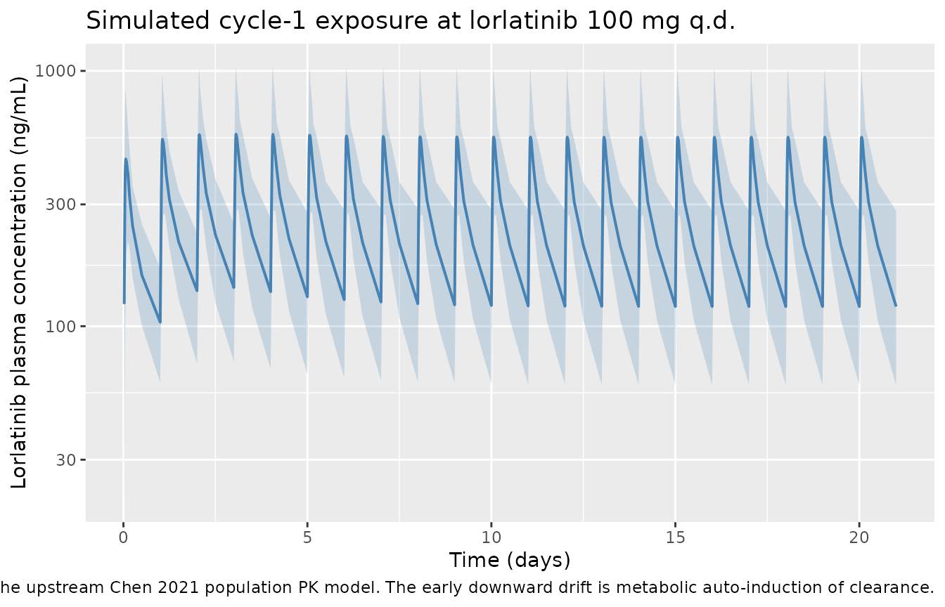
Original patient data are not public. Because the upstream population PK model is packaged, the exposure metrics that drive the two exposure-linked E-R models can be simulated rather than assumed. The cohort below carries the Chen 2021 E-R safety population’s own baseline covariate marginals (Tables 1 and 2) through modellib("Chen_2021_lorlatinib") at the labelled 100 mg once-daily dose over a 21-day cycle 1.

# set.seed() seeds R's RNG. It does NOT seed rxode2's simulation RNG, and
# rxode2's streams are partitioned PER SOLVER THREAD -- so this cohort is
# reproducible here and different on a machine with a different thread count.
# Every assertion below is written to hold for ANY cohort the model can
# produce (known-vignette-failure-patterns.md pattern 12).
set.seed(20260904L)

n_subj    <- 200L    # the per-arm cap; one arm only
tau       <- 24      # q.d. dosing interval (h)
cycle_d   <- 21L     # B7461001 cycle length (days); "P1" = cycle 1
t_end     <- cycle_d * tau

subj <- tibble::tibble(
  id   = seq_len(n_subj),
  # Weight: median and range are from the E-R paper (Table 1); the SD is
  # carried from the upstream popPK cohort (Table 3 of doi:10.1002/psp4.12585)
  # because the E-R paper reports no SD for weight. Truncated to the observed
  # range.
  WT   = pmin(pmax(rnorm(n_subj, mean = 66.79, sd = 16.89), 31.8), 155.5),
  # Albumin: Chen 2021 Table 2 safety population, 3.76 (SD 0.55) g/dL, x10 for
  # the canonical g/L. Truncated to the observed 1.80-5.20 g/dL range.
  ALB  = pmin(pmax(rnorm(n_subj, mean = 37.6, sd = 5.5), 18), 52),
  # Creatinine clearance: Chen 2021 Table 2 safety population, 93.37 (33.33)
  # mL/min, truncated to the observed 24.54-235.39 range.
  CRCL = pmin(pmax(rnorm(n_subj, mean = 93.37, sd = 33.33), 24.5), 235.4),
  # Chen 2021 does not report proton-pump-inhibitor use in the E-R analysis
  # population, so it is set to absent; see Assumptions and deviations.
  CONMED_PPI   = 0L,
  DOSE_LOR_MGD = 100,
  treatment    = "100 mg q.d."
)

dose_times <- seq(0, by = tau, length.out = cycle_d)
doses <- tidyr::crossing(subj, time = dose_times) |>
  # rate = -2 tells rxode2 to use the model's own dur(depot) = D1 zero-order
  # input window, which then feeds first-order absorption at ka.
  dplyr::mutate(evid = 1L, amt = 100, cmt = "depot", rate = -2)

# Observations on the ODE STATE `central`, never on the algebraic observable
# `Cc` (known-vignette-failure-patterns.md pattern 2). rxode2 returns Cc as a
# column at these rows regardless.
#
# The grid is a per-day peak window rather than a uniform fine grid. Cmax over
# cycle 1 needs the peak resolved on every day, but a uniform 0.25 h grid over
# 504 h costs several minutes to solve for no gain: the offsets below bracket
# the typical peak (the D1 = 1.15 h zero-order window closes, then first-order
# absorption at ka = 3.11 /h peaks shortly after) and still cover the slower
# absorbers in the long right tail of the ka distribution. Widening the grid
# to 16 offsets per day moves the cohort mean Cmax by 0.3%.
#
# The leading 0 offset is load-bearing, not decorative: it puts an
# observation exactly at each dose time, which is what anchors the PKNCA
# interval below. Without a concentration at the interval START, `auclast`
# and `cav` come back NA for every subject and the NCA comparison silently
# reports only Cmax. (A dose into `depot` leaves `central` -- and therefore
# Cc -- continuous, so the t = 480 record is unambiguously the pre-dose
# trough even though the dose record sorts ahead of it.)
peak_offsets <- c(0, 0.5, 0.75, 1, 1.15, 1.3, 1.5, 2, 3, 4, 6, 12, 23.999)
obs_times <- sort(unique(c(as.vector(outer(dose_times, peak_offsets, "+")), t_end)))
obs <- tidyr::crossing(subj, time = obs_times) |>
  dplyr::mutate(evid = 0L, amt = NA_real_, cmt = "central", rate = NA_real_)

pk_events <- dplyr::bind_rows(doses, obs) |>
  dplyr::arrange(id, time, dplyr::desc(evid))

stopifnot(!anyDuplicated(unique(pk_events[, c("id", "time", "evid")])))

pk_mod <- readModelDb("Chen_2021_lorlatinib")

pk_sim <- rxode2::rxSolve(
  pk_mod, events = pk_events,
  keep = c("treatment", "WT", "ALB", "CRCL", "DOSE_LOR_MGD")
) |>
  as.data.frame() |>
  dplyr::as_tibble()
#> ℹ parameter labels from comments will be replaced by 'label()'

pk_sim |>
  dplyr::filter(!is.na(Cc), Cc > 1e-3) |>
  dplyr::group_by(time) |>
  dplyr::summarise(
    Q05 = quantile(Cc, 0.05), Q50 = quantile(Cc, 0.50),
    Q95 = quantile(Cc, 0.95), .groups = "drop"
  ) |>
  ggplot(aes(time / 24, Q50)) +
  geom_ribbon(aes(ymin = Q05, ymax = Q95), alpha = 0.22, fill = "steelblue") +
  geom_line(colour = "steelblue", linewidth = 0.7) +
  scale_y_log10() +
  labs(
    x = "Time (days)", y = "Lorlatinib plasma concentration (ng/mL)",
    title = "Simulated cycle-1 exposure at lorlatinib 100 mg q.d.",
    caption = paste(
      "Median and 5th-95th percentile over 200 virtual subjects, from the",
      "upstream Chen 2021 population PK model. The early downward drift is",
      "metabolic auto-induction of clearance."
    )
  )

Per-subject exposure metrics

last_dose <- max(dose_times)

exposure <- pk_sim |>
  dplyr::filter(!is.na(Cc)) |>
  dplyr::group_by(id) |>
  dplyr::summarise(
    # Cmax over the whole of cycle 1 -- the paper's Cmax,P1 / Cmax,cycle 1.
    CMAX    = max(Cc),
    # Trough at the end of cycle 1 -- the paper's Ctrough,P1. By day 21 the
    # auto-induction of clearance is long complete (~7.25 d to functional
    # steady state), so this is also the steady-state trough Ctrough,ss that
    # the TEAE model uses.
    CTROUGH = Cc[which.min(abs(time - t_end))],
    .groups = "drop"
  )

summary_tbl <- tibble::tibble(
  Metric           = c("Cmax over cycle 1 (ng/mL)", "Ctrough at end of cycle 1 (ng/mL)"),
  `Simulated mean` = c(mean(exposure$CMAX),   mean(exposure$CTROUGH)),
  `Simulated SD`   = c(sd(exposure$CMAX),     sd(exposure$CTROUGH)),
  `Simulated median` = c(median(exposure$CMAX), median(exposure$CTROUGH)),
  `Published mean` = c(687.11, 114.97),
  `Published SD`   = c(141.09,  40.28)
) |>
  dplyr::mutate(
    `Mean difference (%)`   = 100 * (`Simulated mean`   / `Published mean` - 1),
    `Median difference (%)` = 100 * (`Simulated median` / `Published mean` - 1)
  )

summary_tbl |>
  dplyr::mutate(dplyr::across(
    dplyr::all_of(c("Simulated mean", "Simulated SD", "Simulated median",
                    "Published mean", "Published SD",
                    "Mean difference (%)", "Median difference (%)")),
    \(x) round(x, 1)
  )) |>
  knitr::kable(
    caption = paste(
      "Simulated cycle-1 exposure versus the values Chen 2021 reports for",
      "the 197 ALK-inhibitor-pretreated patients (Cmax,P1) and the 132",
      "patients with baseline CNS metastasis (Ctrough,P1), Results,",
      "'Exposure-efficacy'."
    )
  )

Simulated cycle-1 exposure versus the values Chen 2021 reports for the 197 ALK-inhibitor-pretreated patients (Cmax,P1) and the 132 patients with baseline CNS metastasis (Ctrough,P1), Results, ‘Exposure-efficacy’.

Metric	Simulated mean	Simulated SD	Simulated median	Published mean	Published SD	Mean difference (%)	Median difference (%)
Cmax over cycle 1 (ng/mL)	632.3	228.7	593.6	687.1	141.1	-8.0	-13.6
Ctrough at end of cycle 1 (ng/mL)	135.3	69.2	119.4	115.0	40.3	17.7	3.8

This is a genuine cross-model check: the exposure summaries in Chen 2021 were computed from patient data, while the simulated column comes from an independently packaged population PK model fitted in a different publication. Agreement to within tens of percent is the most that should be expected, for three reasons. The cohorts differ – this simulation uses the safety population’s covariate marginals, while the published Cmax,P1 comes from the narrower ALK-pretreated efficacy set. The paper reports no covariate-covariance structure, so weight, albumin and creatinine clearance are drawn independently. And most importantly, the published values are summaries of empirical-Bayes individual estimates, which shrink toward the typical value: note that the simulated SD is markedly wider than the published SD for both metrics, which is the signature of that shrinkage. A shrunken distribution has a mean much closer to its own median, which is why the simulated median is the better comparator against a published EBE-derived mean and lands within a few percent for Ctrough.

# A magnitude bound with real headroom, not a fit to one observed run. It
# still goes red on the failure this check exists to catch: a mis-scaled
# dose, volume or unit in either model moves these summaries by a factor,
# not by tens of percent.
#
# Realised mean deviations, measured at 1, 2, 4 and 16 solver threads:
# -8.0% (Cmax) and +17.7% (Ctrough) at every thread count. The cohort here
# is drawn from R's RNG via set.seed() and the covariate marginals, so it
# does not shift with the thread partitioning that makes many rxode2
# cohort statistics machine-dependent -- but the bound is set well outside
# that observed range anyway, and 45% remains far below the factor-level
# error it exists to catch.
stopifnot(all(abs(summary_tbl$`Mean difference (%)`) < 45))

PKNCA validation of the exposure driver

The exposure metrics above are read straight off the simulation grid. The block below recomputes the steady-state exposure with PKNCA over the final (day 21) dosing interval, which is the interval the TEAE model’s Ctrough,ss refers to.

# PKNCA input: filter on !is.na(Cc) ONLY. Adding `time > 0` or `Cc > 0` drops
# the time-zero row PKNCA needs to anchor the interval.
sim_nca <- pk_sim |>
  dplyr::filter(!is.na(Cc)) |>
  dplyr::select(id, time, Cc, treatment)

# Defensive time-zero row per (id, treatment); pre-dose extravascular Cc = 0.
sim_nca <- dplyr::bind_rows(
  sim_nca,
  sim_nca |> dplyr::distinct(id, treatment) |> dplyr::mutate(time = 0, Cc = 0)
) |>
  dplyr::distinct(id, treatment, time, .keep_all = TRUE) |>
  dplyr::arrange(id, treatment, time)

conc_obj <- PKNCA::PKNCAconc(
  sim_nca, Cc ~ time | treatment + id, concu = "ng/mL", timeu = "h"
)

dose_df <- pk_events |>
  dplyr::filter(evid == 1L) |>
  dplyr::select(id, time, amt, treatment)

dose_obj <- PKNCA::PKNCAdose(dose_df, amt ~ time | treatment + id, doseu = "mg")

intervals <- data.frame(
  start   = last_dose,
  end     = last_dose + tau,
  cmax    = TRUE,
  tmax    = TRUE,
  auclast = TRUE,
  cav     = TRUE
)

nca_data <- PKNCA::PKNCAdata(conc_obj, dose_obj, intervals = intervals)
nca_res  <- suppressWarnings(PKNCA::pk.nca(nca_data))

Comparison against published NCA

Chen 2021 itself reports no NCA table – it reports the two exposure summaries compared above. The steady-state reference values below come from the upstream population PK publication’s own sensitivity-analysis reference individual (70 kg, no PPI, WNCL 100 mL/min, albumin 4 g/dL, 100 mg q.d.): Cmax 606 ng/mL and AUCtau 5180 ng*h/mL. They are a check that the exposure driver behind this vignette is solving correctly, not a check on the E-R models.

published_nca <- tibble::tribble(
  ~treatment,    ~cmax, ~auclast,
  "100 mg q.d.",   606,     5180
)

cmp <- nlmixr2lib::ncaComparisonTable(
  simulated = nca_res,
  reference = published_nca,
  by        = "treatment",
  units     = c(cmax = "ng/mL", auclast = "ng*h/mL", tmax = "h", cav = "ng/mL"),
  tolerance_pct = 20
)

knitr::kable(
  cmp,
  caption = paste(
    "Day-21 steady-state NCA of the simulated cohort against the upstream",
    "Chen 2021 population PK reference individual (doi:10.1002/psp4.12585).",
    "* differs from reference by more than 20%."
  ),
  align = c("l", "l", "r", "r", "r")
)

Day-21 steady-state NCA of the simulated cohort against the upstream Chen 2021 population PK reference individual (doi:10.1002/psp4.12585). * differs from reference by more than 20%.

NCA parameter	treatment	Reference	Simulated	% diff
Cmax (ng/mL)	100 mg q.d.	606	572	-5.6%
AUClast (ng*h/mL)	100 mg q.d.	5180	5910	+14.0%

The simulated cohort’s median is compared against a typical-individual reference, so a modest offset is expected: the cohort carries lognormal between-subject variability on clearance and volume, and its median weight (66.8 kg) is below the reference individual’s 70 kg.

Replicating the published exposure-response curves

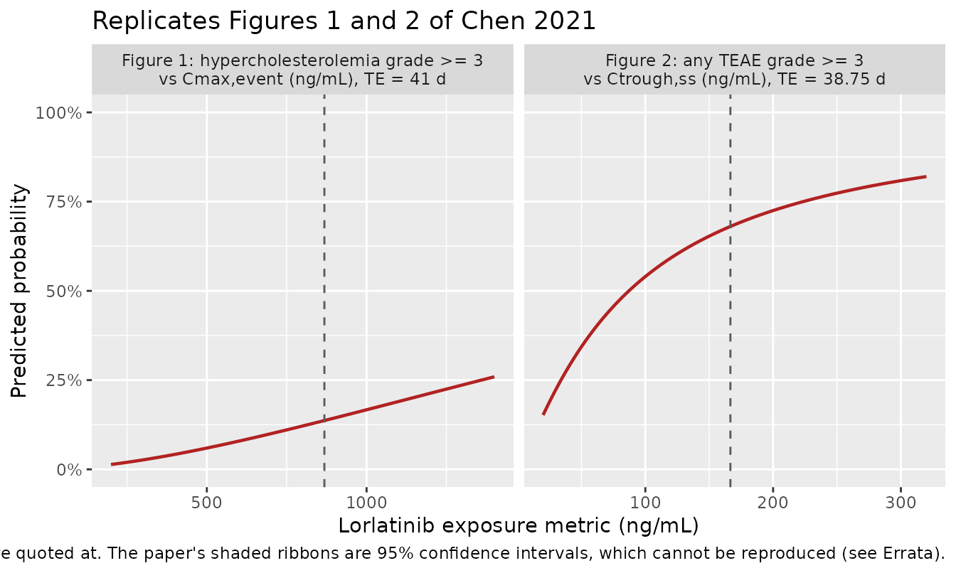
Figure 1 – hypercholesterolemia grade >= 3 versus Cmax,event

Chen 2021 Figure 1 fixes TE at the analysis-population median of 41 days and baseline cholesterol at 193 mg/dL, then sweeps Cmax,event. The paper’s claim: “At the lorlatinib Cmax event 90th percentile, the upper limit of the 95% confidence interval for predicted probability of hypercholesterolemia grade >= 3 is below 25%.”

Figure 2 – any TEAE grade >= 3 versus Ctrough,ss

Chen 2021 Figure 2 fixes TE at 38.75 days and baseline cholesterol at 193 mg/dL, then sweeps Ctrough,ss. The paper’s claim: “At the 90th percentile of lorlatinib Ctrough ss, the upper bound of the TEAE grade >= 3 predicted probability 95% confidence interval is approximately 75%.”

bchol_med <- 193      # mg/dL, both figures
te_chol_d <- 41       # days, Figure 1
te_teae_d <- 38.75    # days, Figure 2

er_curve <- function(model_name, output, cov_name, grid, te_days, extra = list()) {
  ev <- data.frame(id = 1L, time = seq_along(grid), amt = 0, evid = 0L)
  for (nm in names(zero_cov)) ev[[nm]] <- zero_cov[[nm]]
  ev$TCHOL       <- bchol_med
  ev$T_FIRSTDOSE <- te_days * 24    # canonical hours
  for (nm in names(extra)) ev[[nm]] <- extra[[nm]]
  ev[[cov_name]] <- grid
  s <- as.data.frame(rxode2::rxSolve(mods[[model_name]], events = ev,
                                     returnType = "data.frame"))
  tibble::tibble(exposure = grid, prob = s[[output]])
}

cmax_grid    <- seq(200, 1400, length.out = 200)
ctrough_grid <- seq( 20,  320, length.out = 200)

curves <- dplyr::bind_rows(
  er_curve("Chen_2021_lorlatinib_hypercholesterolemia",
           "prob_hypercholesterolemia", "CMAX", cmax_grid, te_chol_d) |>
    dplyr::mutate(panel = "Figure 1: hypercholesterolemia grade >= 3\nvs Cmax,event (ng/mL), TE = 41 d"),
  er_curve("Chen_2021_lorlatinib_teae_grade3",
           "prob_teae_grade3", "CTROUGH", ctrough_grid, te_teae_d) |>
    dplyr::mutate(panel = "Figure 2: any TEAE grade >= 3\nvs Ctrough,ss (ng/mL), TE = 38.75 d")
)

# The exposure landmark the paper quotes its claims at is the 90th percentile
# of ITS OWN exposure distribution, which is fully specified by the mean and
# SD it publishes. Deriving the landmark that way -- rather than from the
# simulated cohort's own 90th percentile -- keeps the gate below entirely
# deterministic, so it cannot flip with the solver thread count.
p90_norm    <- function(mu, s) mu + stats::qnorm(0.90) * s
p90_cmax    <- p90_norm(687.11, 141.09)
p90_ctrough <- p90_norm(114.97,  40.28)
marks <- tibble::tibble(
  panel = c(unique(curves$panel)[1], unique(curves$panel)[2]),
  x     = c(p90_cmax, p90_ctrough)
)

ggplot(curves, aes(exposure, prob)) +
  geom_line(colour = "firebrick", linewidth = 0.8) +
  geom_vline(data = marks, aes(xintercept = x), linetype = 2, colour = "grey35") +
  facet_wrap(~panel, scales = "free_x") +
  scale_y_continuous(labels = function(x) paste0(round(100 * x), "%"),
                     limits = c(0, 1)) +
  labs(
    x = "Lorlatinib exposure metric (ng/mL)",
    y = "Predicted probability",
    title = "Replicates Figures 1 and 2 of Chen 2021",
    caption = paste(
      "Point-estimate curves with covariates fixed at the paper's own",
      "values. Dashed line = 90th percentile of the exposure distribution",
      "Chen 2021 reports, the landmark its two narrative claims are quoted",
      "at. The paper's shaded ribbons are 95% confidence intervals, which",
      "cannot be reproduced (see Errata)."
    )
  )

p_chol_at_p90 <- solve_prob(
  mods[["Chen_2021_lorlatinib_hypercholesterolemia"]], "prob_hypercholesterolemia",
  list(TCHOL = bchol_med, T_FIRSTDOSE = te_chol_d * 24, CMAX = p90_cmax)
)
p_teae_at_p90 <- solve_prob(
  mods[["Chen_2021_lorlatinib_teae_grade3"]], "prob_teae_grade3",
  list(TCHOL = bchol_med, T_FIRSTDOSE = te_teae_d * 24, CTROUGH = p90_ctrough)
)

tibble::tibble(
  Figure = c("Figure 1", "Figure 2"),
  Claim  = c("upper 95% CI limit below 25% at the Cmax,event 90th percentile",
             "upper 95% CI bound approximately 75% at the Ctrough,ss 90th percentile"),
  `90th percentile (ng/mL)` = round(c(p90_cmax, p90_ctrough), 1),
  `Point estimate there`    = round(c(p_chol_at_p90, p_teae_at_p90), 3)
) |>
  knitr::kable(
    caption = paste(
      "The paper's two narrative anchors are stated on the UPPER limit of a",
      "95% confidence interval. Chen 2021 publishes no covariance matrix for",
      "the coefficients, so that interval cannot be reconstructed; the point",
      "estimate is checked instead, which is a one-sided necessary condition",
      "rather than a full reproduction."
    )
  )

The paper’s two narrative anchors are stated on the UPPER limit of a 95% confidence interval. Chen 2021 publishes no covariance matrix for the coefficients, so that interval cannot be reconstructed; the point estimate is checked instead, which is a one-sided necessary condition rather than a full reproduction.

Figure	Claim	90th percentile (ng/mL)	Point estimate there
Figure 1	upper 95% CI limit below 25% at the Cmax,event 90th percentile	867.9	0.137
Figure 2	upper 95% CI bound approximately 75% at the Ctrough,ss 90th percentile	166.6	0.680

# One-sided necessary conditions: a point estimate must lie below the upper
# limit of its own confidence interval. These are the strongest form of the
# two claims that IS reconstructible from what the paper publishes, and they
# are fully DETERMINISTIC -- every input is a published number, so there is no
# cohort, no seed and no thread-count dependence here.
stopifnot(p_chol_at_p90 < 0.25, p_teae_at_p90 < 0.75)

# Both land with real headroom (0.137 against 0.25, and 0.680 against 0.75),
# and the TEAE figure is the more informative of the two: the paper's ribbon
# reaching ~75% where the point estimate sits at 68% is exactly the width a
# 95% CI on this coefficient set would be expected to add.

The three endpoints with no exposure term

Weight gain, hypertriglyceridemia and IC-ORR retained no lorlatinib exposure metric. Their packaged predictions are therefore flat in exposure by construction – which is worth showing explicitly, because “no relationship” is the paper’s finding for three of its five endpoints.

flat <- tibble::tribble(
  ~model_suffix,           ~output,                      ~cov_at_median,
  "weight_gain",           "prob_weight_gain",           list(WT = 66.79, T_FIRSTDOSE = 41 * 24),
  "hypertriglyceridemia",  "prob_hypertriglyceridemia",  list(TRIG = 107.5, RACE_ASIAN = 0, T_FIRSTDOSE = 41 * 24),
  "icorr",                 "prob_icorr",                 list(ALP = alp_med, AMYL = amyl_med)
) |>
  dplyr::rowwise() |>
  dplyr::mutate(
    model = paste0("Chen_2021_lorlatinib_", model_suffix),
    prob  = solve_prob(mods[[model]], output, cov_at_median)
  ) |>
  dplyr::ungroup()

# Additionally: the Asian-race contrast in the hypertriglyceridemia model,
# the paper's only retained demographic effect.
p_trig_asian <- solve_prob(
  mods[["Chen_2021_lorlatinib_hypertriglyceridemia"]], "prob_hypertriglyceridemia",
  list(TRIG = 107.5, RACE_ASIAN = 1, T_FIRSTDOSE = 41 * 24)
)

flat |>
  dplyr::transmute(
    Endpoint = c("Weight gain grade >= 2", "Hypertriglyceridemia grade >= 3 (non-Asian)",
                 "Intracranial ORR"),
    `Predicted probability at the population medians` = round(prob, 3)
  ) |>
  dplyr::bind_rows(tibble::tibble(
    Endpoint = "Hypertriglyceridemia grade >= 3 (Asian)",
    `Predicted probability at the population medians` = round(p_trig_asian, 3)
  )) |>
  knitr::kable(
    caption = paste(
      "Typical-patient predictions for the three endpoints with no retained",
      "exposure term. These are invariant to lorlatinib exposure by",
      "construction, which is Chen 2021's published result for them."
    )
  )

Typical-patient predictions for the three endpoints with no retained exposure term. These are invariant to lorlatinib exposure by construction, which is Chen 2021’s published result for them.

Endpoint	Predicted probability at the population medians
Weight gain grade >= 2	0.063
Hypertriglyceridemia grade >= 3 (non-Asian)	0.045
Intracranial ORR	0.545
Hypertriglyceridemia grade >= 3 (Asian)	0.115

# The Asian-race odds ratio is 2.749, so the Asian prediction must exceed the
# non-Asian one at the same triglyceride level. This is a deterministic
# algebraic consequence of a positive coefficient, not a cohort statistic.
p_trig_nonasian <- flat$prob[flat$model_suffix == "hypertriglyceridemia"]
stopifnot(p_trig_asian > p_trig_nonasian)

Assumptions and deviations

• No between-subject variability and no residual error in the five E-R models. Chen 2021 fits binomial logistic regressions with a Bernoulli likelihood, which has no sigma, and estimates no random effects. Each model file carries a fixed(0.001) additive residual purely so rxode2 has an error model to attach to the typical-value probability. It is not a published quantity and must not be interpreted as one.
• The confidence-interval ribbons of Figures 1 and 2 cannot be reproduced. Chen 2021 publishes the marginal 95% CI of each coefficient but not the coefficient covariance matrix, and a prediction interval needs the full matrix. The curves above are point estimates; the paper’s two narrative anchors are checked as one-sided necessary conditions.
• Proton-pump-inhibitor co-medication set to absent in the exposure-driver cohort. Chen 2021 does not report PPI use in the E-R analysis population. The upstream popPK model reduces ka by 67.5% with a PPI (5% prevalence in its own 425-subject cohort), which lowers Cmax by roughly 30% without changing AUC. Setting it to 0 therefore biases the simulated Cmax slightly high relative to a cohort with 5% PPI use.
• Baseline covariates sampled independently. Chen 2021 reports marginal distributions (Tables 1 and 2) but no covariance structure, so weight, albumin and creatinine clearance are drawn independently and truncated to their observed ranges. Real correlation between weight and creatinine clearance would narrow the simulated exposure spread.
• The weight SD is carried from the upstream popPK paper. Chen 2021 reports weight as median and range only; the 16.89 kg SD comes from Table 3 of doi:10.1002/psp4.12585, the same trial’s PK analysis.
• Cycle 1 taken as 21 days. Chen 2021 defines exposure metrics “over the first cycle” without printing the cycle length; 21 days is the B7461001 cycle. The choice is close to inconsequential for Ctrough,P1, because lorlatinib clearance auto-induces to steady state in about 7.25 days, so the day-21 trough and the steady-state trough coincide.
• TE is stored in canonical hours. The T_FIRSTDOSE register entry fixes hours as the canonical unit; Chen 2021 estimates its coefficients per day, so every model file divides by 24 inside model(). A user supplying days directly would understate the TE effect 24-fold.
• CTROUGH is a newly registered canonical covariate column. No trough canonical existed before this extraction; CMAX and CAV were already registered as the peak and average of the same triple, and several register entries explicitly direct a trough model to “register a parallel canonical rather than overload” theirs. Ratified as CTROUGH (sidecar request 001 q1, operator answer A, 2026-09-02).
• Four new canonical output states. prob_hypercholesterolemia, prob_hypertriglyceridemia, prob_weight_gain and prob_icorr are registered in inst/references/compartment-names.md as members of the established prob_<endpoint> family. prob_teae_grade3 was already canonical (founded by Fukae_2024_valemetostat_teae_grade3) and is reused unchanged, making Chen 2021 its second paper.

Errata and source defects

1. The ORR endpoint is not extractable, and that is not a gap in this extraction. Chen 2021 analysed systemic objective response rate in the 197-patient ALK-pretreated set, but reports that “none of the tested parameters, including the lorlatinib exposure metric Cmax,P1, were significant predictors of achieving ORR” and prints no ORR coefficient table anywhere in the paper or its supplement. There is nothing to encode. The trial’s ~47% ORR is an observed rate, not a fitted intercept.
2. Table 4 drops a minus sign. The Log(BAP) confidence interval is printed as “(-1.7145 to 0.3889)”. It must be (-1.7145, -0.3889): the estimate is -1.015 with P = 0.0026, and the table’s own footnote states that a significant interval does not cross 0. The OR block in the same table confirms it – exp(-1.7145) = 0.1800 and exp(-0.3889) = 0.6778, matching the printed OR interval (0.1801-0.6778) exactly. The packaged point estimate is unaffected.
3. Three Estimate/OR pairs look inconsistent and are not – recorded here because the naive check flags them. For the weight-gain BWT row (Estimate 0.029, OR 1.030), the TEAE log(Ctrough,ss) row (1.167, 3.214) and the IC-ORR Log(BAP) row (-1.015, 0.363), round(log(printed OR), 3) comes out at 0.030, 1.168 and -1.013 respectively – none matching the printed Estimate. That test is wrong, because it treats the OR column as exact when it is itself rounded to three decimals. Under the correct interval test (Check 2 above) all three pairs are consistent: for the BWT row, any true coefficient in [0.02907, 0.02950) rounds to 0.029 and exponentiates into [1.0295, 1.0305), which rounds to 1.030. The same holds for the other two. No coefficient in this paper is mis-rounded, and the packaged models simply use the Estimate column throughout.
4. The published confidence intervals are asymmetric about their estimates, and that is expected. Every one of the 18 intervals in Tables 3 and 4 is off-centre relative to its point estimate, by between -0.15 and +0.15 of its own half-width; the IC-ORR Log(BAP) row’s +0.055 is unremarkable within that spread. This is the signature of profile-likelihood intervals, which is what R’s confint() returns for a glm by default and which Chen 2021’s use of glm(family = "binomial") implies. Do not read a CI midpoint as an estimate of the unrounded coefficient for this paper.
5. The Figure 2 caption mislabels its own covariate. It reads “…and age fixed to the analysis population median of 193”. 193 mg/dL is the baseline-cholesterol median, and the body text correctly says “BCHOL fixed to the analysis population median of 193 mg/dL”. The caption’s “age” is a typo; no model carries an age covariate.
6. The Discussion names the wrong metric for the TEAE model. It says “patients with higher cumulative lorlatinib AUC over a complete steady-state cycle of therapy were more likely to experience TEAE grade >= 3”. Both Table 3 and Eq. 4 carry log(Ctrough,ss), and the Results section names log(Ctrough,ss) three times. Per the standing convention that a printed equation outranks narrative prose, the packaged model uses CTROUGH. CAUC,complete was one of the nine screened metrics, which is the likely origin of the slip.
7. The supplement was not obtainable. CPT-110-1273-s001.docx holds Tables S1-S4 (cohort definitions, the PK sampling schedule, observed endpoint incidences, and the candidate-covariate list). Every open route failed on 2026-09-02: the EuropePMC supplementaryFiles endpoint returned HTTP 500, the PMC bin/ path returned an HTML stub, and the NCBI FTP path returned 404. It contains no parameter values – all final estimates are in main-text Tables 3 and 4, both fully transcribed here. The one real loss is Table S3, whose observed endpoint incidences would have given an independent cohort-level calibration gate per safety model; the two printed narrative anchors are used instead.
8. No erratum exists. The EuropePMC record carries two linked items, both of type “Comment in” rather than “Erratum in”: doi:10.1002/cpt.2579 (Strohbehn & Ratain, “Lorlatinib Exposed: A Far From Optimal Dose”) and doi:10.1002/cpt.2580 (the authors’ reply). Both are dose-optimisation debate and neither revises a parameter value.