Mycophenolic acid (Suzuki 2024)
Source:vignettes/articles/Suzuki_2024_mycophenolic_acid.Rmd
Suzuki_2024_mycophenolic_acid.RmdModel and source
- Citation: Suzuki Y, Matsunaga N, Aoyama T, Ogami C, Hasegawa C, Iida S, To H, Kitahara T, Tsuji Y. (2024). Population pharmacokinetic analysis identifies an absorption process model for mycophenolic acid in patients with renal transplant. Clin Transl Sci 17(12):e70097. doi:10.1111/cts.70097
- Description: Population pharmacokinetic model for mycophenolic acid (MPA), the active metabolite of mycophenolate mofetil (MMF), in 42 adult renal transplant recipients at a single Japanese centre (312 plasma MPA observations from 14 days pre- to 84 days post-transplantation; MMF 500-1000 mg twice daily). The paper compared six absorption structures plus an enterohepatic-circulation (EHC) model; a two-compartment disposition model with SEQUENTIAL zero- then first-order absorption and a lag time gave the lowest OFV, and the EHC process did not improve the fit. Dose enters the depot as a zero-order input over D1 = 1.95 h beginning after a lag of 0.283 h, then drains first-order with ka = ln(2)/TABS (absorption half-life TABS = 0.0453 h, so ka = 15.3 /h and absorption is rate-limited by D1). Apparent total clearance is split into an additive non-renal arm (7.56 L/h) plus a renal arm (11.6 L/h) that scales linearly with renal function RF = CLcr / 100, where CLcr is a Cockcroft-Gault estimate standardised to a 70 kg body weight. Allometric size scaling uses the Holford normal-fat-mass (NFM) framework, but Ffat was estimated as not different from 1 and fixed there for both clearance and volume, so NFM collapses exactly to total body weight and the size model reduces to (WT/70)^0.75 on CL/F and Q/F and (WT/70)^1 on VC/F and VP/F (the paper’s own Equation 8). Post-transplantation day acts on relative bioavailability as F1 = exp(0.956 * POD / 84) for POD >= 0 (1 otherwise), a 2.8-fold rise in exposure by 90 days. The MMF-to-MPA molecular-weight ratio 320.3/433.5 is carried inside F1, so doses are given as mg of MMF. Between-subject variability is exponential on CL/F, VC/F, TABS, lag time and D1, and additive-proportional on F1; BSV on Q/F and VP/F was fixed to zero. Residual error is combined proportional (28.3%) plus additive (0.0634 mg/L).
- Article: https://doi.org/10.1111/cts.70097
- Supplement (Table S1, Figures S1-S2, Appendix S1 NM-TRAN control stream): published with the open-access article (PMC11615510).
Suzuki 2024 asks a specific question: does the well-known “second peak” in mycophenolic acid (MPA) profiles require an explicit enterohepatic-circulation (EHC) compartment, or can the complex, highly variable PK of MPA be captured by a richer absorption model instead? The authors fitted six absorption structures and an EHC model to the same data and let the objective function value (OFV) decide.
The answer was the absorption model. Table S1 of the supplement gives the model development ladder; the sequential zero- then first-order absorption model with a lag time reached the lowest structural OFV (735.671), well below first-order with lag (817.358), zero-order (820.463), the parallel forms (806-825), and both transit-compartment variants (741.759 for the Savic estimated-number model, 751.816 at best for the fixed-number Erlang models). Adding an EHC process did not significantly improve the OFV. The final model (Table S1 row 23, OFV 696.79) added three covariate effects to that structure: allometric total body weight on clearances and volumes, renal function on the renal clearance arm, and post-transplantation day on relative bioavailability.
Structure
The packaged model is a two-compartment disposition model fed by a
depot that receives the dose as a zero-order input of duration
d1, beginning after a lag tlag, and
then drains first-order at ka:
dose --(lag 0.283 h)--> [ zero-order input over 1.95 h ] --> depot --ka--> central <--> peripheral1
                                                                             |
                                                                            CL/F
Because the fitted absorption half-life is very short (TABS = 0.0453
h, so ka = ln(2)/TABS = 15.3 /h, a 2.7-minute half-life),
the first-order step is effectively instantaneous and the
rate-limiting part of absorption is the 1.95 h zero-order
input. That is what produces the flat-topped, slightly delayed peak this
model predicts, and the very large between-subject variability on the
lag time (121.7% CV) is what lets it also describe the markedly delayed
profiles visible in Suzuki 2024 Figure 1.
Three further features are worth calling out because they are easy to get wrong when reading the paper alone:
-
Clearance is split into two additive arms.
CL/F = CL_nonrenal/F + CL_renal/F * RF(Equation 5), whereRF = CLcr / 100(Equation 4). A single between-subject random effect acts on the composite, not on the two arms separately (Appendix S1 buildsGRPCLfirst and only then appliesEXP(PPV_CL)). -
The size model collapses to plain body weight. The
paper sets up the Holford normal-fat-mass (NFM) descriptor (Equations
1-3), but
Ffatwas estimated as not different from 1 and fixed there for both clearance and volume. WithFfat = 1,NFM = FFM + (TBW - FFM) = TBWandNFMstd = 56.1 + (70 - 56.1) = 70kg exactly, so the whole NFM apparatus reduces to(TBW/70)^0.75on CL/F and Q/F and(TBW/70)^1on VC/F and VP/F. That is how the authors themselves write the final model in Equation 8, and height and sex drop out entirely. -
The dose is mycophenolate mofetil, not MPA. The
MMF-to-MPA molecular-weight ratio 320.3/433.5 = 0.7389 is carried inside
F1(Appendix S1GRPF1 = POP_F1 * MWMPA * FPTD), because MMF is hydrolysed to MPA presystemically. Doses passed to this model are therefore in mg of MMF.
Population
The model was built from 42 adult kidney transplant recipients treated at Nagasaki University Hospital between April 2011 and September 2019, contributing 312 steady-state plasma MPA concentrations collected between 14 days pre-transplantation and 84 days post-transplantation. Twenty-nine were male and 13 female. Baseline characteristics are reported in Suzuki 2024 Table 1 as 2.5th / 50th / 97.5th percentiles rather than mean +/- SD: age 29.0 / 51.0 / 68.9 years, height 1.50 / 1.66 / 1.80 m, total body weight 39.6 / 55.9 / 77.5 kg, post-transplantation day 23 / 40 / 84, and creatinine clearance 6.6 / 52.8 / 148.8 mL/min/70 kg. The cohort is therefore lighter than a typical Western transplant population and spans essentially the whole range of graft function from severe impairment to hyperfiltration.
Mycophenolate mofetil was given twice daily at 500 mg (n = 10), 750 mg (n = 25) or 1000 mg (n = 7). Tacrolimus (n = 24) and prednisone (n = 23) were given concomitantly in some patients; neither improved the OFV as a covariate on CL/F or VC/F and neither appears in the final model.
The same information is available programmatically:
pop <- rxode2::rxode(readModelDb("Suzuki_2024_mycophenolic_acid"))$population
str(pop, max.level = 1)
#> List of 17
#>  $ species       : chr "human"
#>  $ n_subjects    : int 42
#>  $ n_studies     : int 1
#>  $ n_observations: chr "312 plasma MPA concentrations (Suzuki 2024 Results 'PopPK of MPA')"
#>  $ age_range     : chr "29.0-68.9 years (2.5th-97.5th percentile; median 51.0)"
#>  $ age_median    : chr "51.0 years"
#>  $ weight_range  : chr "39.6-77.5 kg (2.5th-97.5th percentile; median 55.9)"
#>  $ weight_median : chr "55.9 kg"
#>  $ height_range  : chr "1.50-1.80 m (2.5th-97.5th percentile; median 1.66)"
#>  $ sex_female_pct: num 31
#>  $ race_ethnicity: chr "not reported; single-centre Japanese cohort"
#>  $ disease_state : chr "adult kidney transplant recipients receiving mycophenolate mofetil immunosuppression"
#>  $ renal_function: chr "creatinine clearance 6.6-148.8 mL/min/70 kg (2.5th-97.5th percentile; median 52.8), i.e. spanning normal to sev"| __truncated__
#>  $ dose_range    : chr "mycophenolate mofetil 500 mg (n = 10), 750 mg (n = 25) or 1000 mg (n = 7) orally twice daily, every 12 h"
#>  $ regions       : chr "Japan (Nagasaki University Hospital, April 2011 to September 2019)"
#>  $ co_medication : chr "tacrolimus (n = 24, median trough 6.9 ug/L) and prednisone (n = 23, median 10 mg/day) in some patients; neither"| __truncated__
#>  $ notes         : chr "Baseline demographics from Suzuki 2024 Table 1 (reported as 2.5th / 50th / 97.5th percentiles rather than mean "| __truncated__
Source trace
The per-parameter origin is recorded as an in-file comment next to
each ini() entry in
inst/modeldb/specificDrugs/Suzuki_2024_mycophenolic_acid.R.
The table below collects them in one place. Every final estimate appears
both in Table 2 (column “Final model estimate”) and in the
$THETA / $OMEGA blocks of the NM-TRAN control
stream reproduced as Appendix S1, and the two agree throughout.
| Equation / parameter | Value | Source location |
|---|---|---|
lcl_nonren (CL_nonrenal/F) |
7.56 L/h | Table 2; Appendix S1 POP_CLNR
|
lcl_renal (CL_renal/F) |
11.6 L/h | Table 2; Appendix S1 POP_CLR
|
lvc (VC/F) |
104.0 L | Table 2; Appendix S1 POP_V2
|
lq (Q/F) |
17.3 L/h | Table 2; Appendix S1 POP_Q
|
lvp (VP/F) |
169.0 L | Table 2; Appendix S1 POP_V3
|
ltabs (TABS) |
0.0453 h | Table 2; Appendix S1 POP_TABS; Eq. 8
ka = 0.693/0.0453
|
ltlag (ALAG1) |
0.283 h | Table 2; Appendix S1 POP_ALAG1
|
ld1 (D1) |
1.95 h | Table 2; Appendix S1 POP_D1
|
lfdepot (F1) |
1, fixed | Table 2 “1 fixed”; Appendix S1 1. FIX ; POP_F1
|
e_wt_cl_q |
0.75, fixed | Methods “Covariate model”; Appendix S1
FSIZCL=...**(3/4); Eq. 8 |
e_wt_vc_vp |
1, fixed | Methods “Covariate model”; Appendix S1 FSIZV=...**1;
Eq. 8 |
e_pod_fdepot (K_PTD) |
0.956 | Table 2; Appendix S1 KPTD; Eq. 6 and Eq. 8 |
etalcl |
0.183 | Appendix S1 $OMEGA ... PPV_CL; Table 2 42.8 CV% |
etalvc |
0.337 | Appendix S1 $OMEGA ... PPV_V2; Table 2 58.1 CV% |
etaltabs |
0.534 | Appendix S1 $OMEGA ... PPV_TABS; Table 2 73.1 CV% |
etaltlag |
1.48 | Appendix S1 $OMEGA ... PPV_ALAG1; Table 2 121.7
CV% |
etald1 |
0.825 | Appendix S1 $OMEGA ... PPV_D1; Table 2 90.8 CV% |
etalfdepot |
0.0324 | Appendix S1 $OMEGA ... PPV_F1; Table 2 18.0 CV% |
propSd |
0.283 | Table 2; Appendix S1 RUV_PROP
|
addSd |
0.0634 mg/L | Table 2; Appendix S1 RUV_ADD
|
Size model (WT/70)^PWR
|
n/a | Equations 1-3; Equation 8; Appendix S1 $PK
|
Renal function RF = CLcr/100
|
n/a | Equation 4; Appendix S1 RF=CLCR/100
|
| Additive clearance arms | n/a | Equation 5; Appendix S1
GRPCL=(GRPCLNR+GRPCLR)*FSIZCL
|
F_PTD = exp(K_PTD * PTD / 84) |
n/a | Equation 6; Appendix S1 IF (PTD.GE.0) ...
|
| MMF-to-MPA conversion 320.3/433.5 | n/a | Methods “PopPK”; Appendix S1 MWMPA=320.3/433.5
|
| Combined residual error | n/a | Appendix S1 $ERROR SD=SQRT(PROP*PROP+ADD*ADD)
|
AUC0-12 = F1 * Dose / (CL_total/F) |
n/a | Equation 7 |
Reading the reported “CV%” correctly
Table 2 reports every between-subject variability as a “CV%”. That
column is 100 * sqrt(omega^2) – the
standard deviation of the eta – and not the exact
lognormal coefficient of variation
100 * sqrt(exp(omega^2) - 1) that much of the popPK
literature (and most other models in this package) uses. The
$OMEGA block in Appendix S1 settles it, because it states
the variances directly:
omega2 <- c(CL = 0.183, VC = 0.337, TABS = 0.534,
            ALAG1 = 1.48, D1 = 0.825, F1 = 0.0324)
published_cv <- c(42.8, 58.1, 73.1, 121.7, 90.8, 18.0)

cv_check <- tibble(
  Parameter = names(omega2),
  `omega^2 (Appendix S1)` = omega2,
  `Table 2 CV%` = published_cv,
  `100*sqrt(omega^2)` = round(100 * sqrt(omega2), 1),
  `100*sqrt(exp(omega^2)-1)` = round(100 * sqrt(exp(omega2) - 1), 1)
)
knitr::kable(cv_check)| Parameter | omega^2 (Appendix S1) | Table 2 CV% | 100*sqrt(omega^2) | 100*sqrt(exp(omega^2)-1) |
|---|---|---|---|---|
| CL | 0.1830 | 42.8 | 42.8 | 44.8 |
| VC | 0.3370 | 58.1 | 58.1 | 63.3 |
| TABS | 0.5340 | 73.1 | 73.1 | 84.0 |
| ALAG1 | 1.4800 | 121.7 | 121.7 | 184.2 |
| D1 | 0.8250 | 90.8 | 90.8 | 113.2 |
| F1 | 0.0324 | 18.0 | 18.0 | 18.1 |
# Fail loudly if the identification ever stops holding.
stopifnot(all(abs(100 * sqrt(omega2) - published_cv) < 0.06))
All six values reproduce exactly under 100*sqrt(omega^2)
and none reproduce under the lognormal formula (which would give 44.8,
63.3, 84.0, 184.2, 113.2 and 18.1). The model file therefore uses the
$OMEGA variances verbatim. Had the usual
log(1 + CV^2) convention been applied instead, the lag-time
variance would have been 0.909 rather than 1.48 – a 39% understatement
of the single largest source of variability in the model.
Virtual cohort
The original patient-level data are not public. Two kinds of virtual cohort are used below.
- A demographic cohort whose total body weight reproduces the Table 1 percentiles, used for the illustrative steady-state profiles.
- Fixed-covariate cohorts matching the design the authors used for their own simulations (Methods “Simulation”): total body weight fixed at 70 kg and CLcr set to 25, 50, 75 or 100 mL/min/70 kg. These are used for every validation gate so that the comparison is against the published simulation exactly.
Cohorts are 200 participants per arm.
set.seed(20241204)

mod <- readModelDb("Suzuki_2024_mycophenolic_acid")

TAU       <- 12     # h, dosing interval
# Doses to steady state. The terminal half-life is ~15 h at CLcr 100 but ~23 h
# at CLcr 25 (lower CL, same volumes), so the worst-case arm sets the
# requirement: 25 doses = 288 h is ~12.6 terminal half-lives there.
N_DOSE    <- 25
T_LASTDOSE <- TAU * (N_DOSE - 1)
N_PER_ARM <- 200L

# Build one arm: q12h MMF dosing into `depot` with rate = -2 so that rxode2
# honours the model-specified zero-order duration dur(depot) <- d1, plus a dense
# observation grid over the final (steady-state) dosing interval on the ODE
# state `central`. Observations are placed on the ODE state, never on the
# algebraic observable `Cc`.
make_arm <- function(n, dose_mmf, crcl, pod, wt = 70, id_offset = 0L, label = NULL) {
  ev <-
    rxode2::et(amt = dose_mmf, ii = TAU, until = T_LASTDOSE, cmt = "depot", rate = -2) |>
    rxode2::et(seq(T_LASTDOSE, T_LASTDOSE + TAU, by = 0.05), cmt = "central") |>
    rxode2::et(id = seq_len(n))
  out <- as.data.frame(ev)
  out$id  <- out$id + id_offset
  out$WT  <- if (length(wt) == 1L) wt else wt[match(out$id - id_offset, seq_len(n))]
  out$CRCL <- crcl
  out$POD  <- pod
  out$dose_mmf <- dose_mmf
  out$arm <- if (is.null(label)) paste0("CLcr ", crcl) else label
  out
}
crcl_levels <- c(25, 50, 75, 100)

events_crcl <- bind_rows(lapply(seq_along(crcl_levels), function(i) {
  make_arm(
    n = N_PER_ARM, dose_mmf = 1000, crcl = crcl_levels[i], pod = 0,
    id_offset = (i - 1L) * N_PER_ARM,
    label = paste0("CLcr ", crcl_levels[i], " mL/min/70 kg")
  )
}))

# IDs must be disjoint across arms or rxSolve silently collapses them into one.
# Check that directly: every id must belong to exactly one arm, and the total
# number of distinct ids must be the full 4 x 200.
ids_per_arm <- tapply(events_crcl$id, events_crcl$arm, function(x) length(unique(x)))
stopifnot(
  all(ids_per_arm == N_PER_ARM),
  length(unique(events_crcl$id)) == length(crcl_levels) * N_PER_ARM
)
Simulation
sim_crcl <- rxode2::rxSolve(
  mod, events_crcl,
  keep = c("WT", "CRCL", "POD", "dose_mmf", "arm")
) |>
  as.data.frame()

sim_crcl$arm <- factor(sim_crcl$arm, levels = paste0("CLcr ", crcl_levels, " mL/min/70 kg"))
range(sim_crcl$Cc)
#> [1]  0.2002648 32.4055179
Steady-state profiles across renal function
prof <- sim_crcl |>
  filter(!is.na(Cc)) |>
  mutate(tad = time - T_LASTDOSE) |>
  group_by(arm, tad) |>
  summarise(
    med = median(Cc), lo = quantile(Cc, 0.10), hi = quantile(Cc, 0.90),
    .groups = "drop"
  )

ggplot(prof, aes(tad, med)) +
  geom_ribbon(aes(ymin = lo, ymax = hi, fill = arm), alpha = 0.20) +
  geom_line(aes(colour = arm), linewidth = 0.8) +
  labs(
    x = "Time after dose (h)", y = "MPA concentration (mg/L)",
    colour = NULL, fill = NULL
  ) +
  theme_bw() +
  theme(legend.position = "bottom")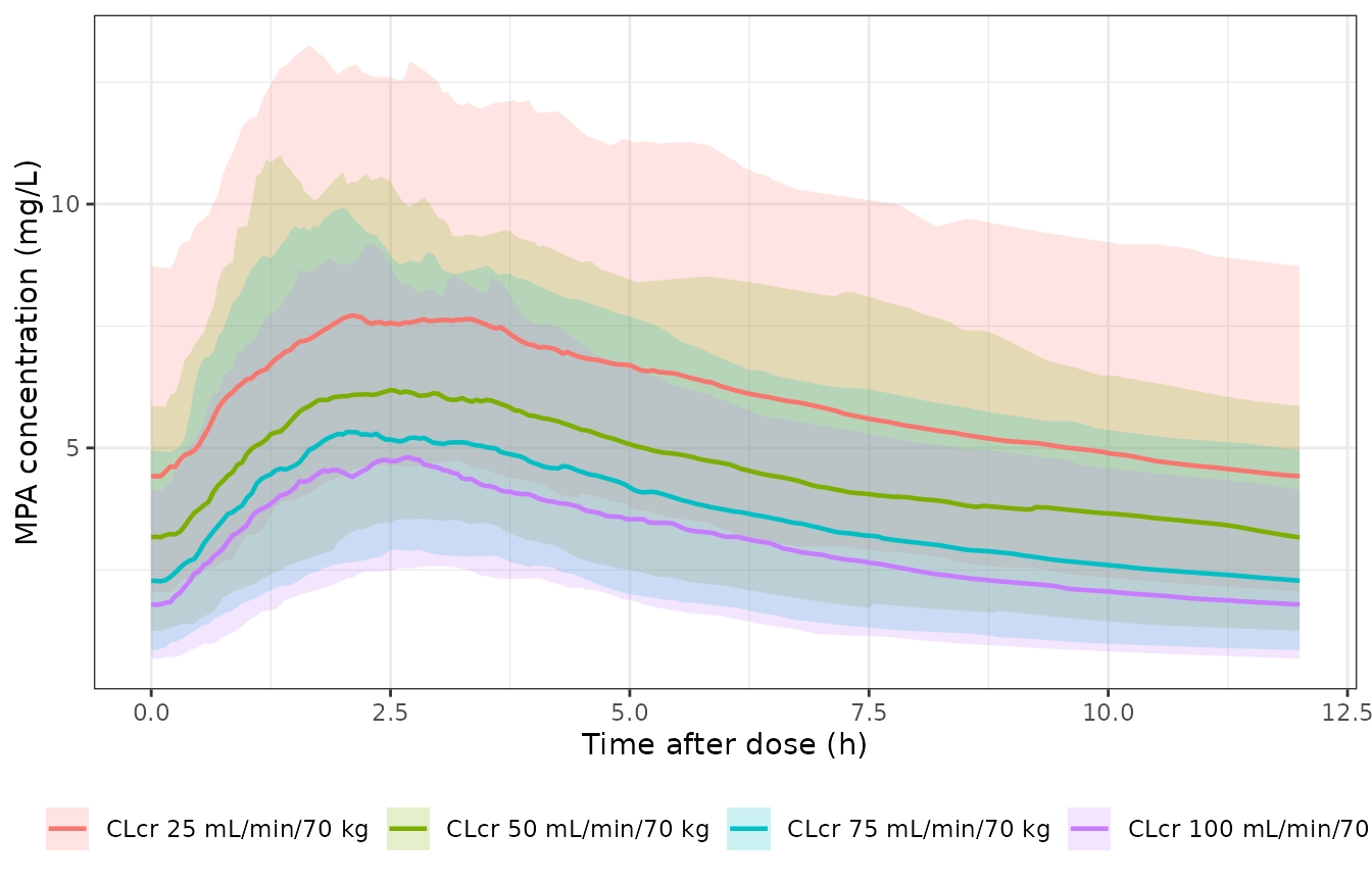
Simulated steady-state MPA concentration-time profiles over the final 12 h dosing interval after MMF 1000 mg twice daily, by renal function. Solid line = median, ribbon = 10th-90th percentile, 200 virtual participants per arm at a fixed 70 kg body weight and post-transplantation day 0.
The shape is the signature of this absorption model. For the
typical individual there is essentially no concentration until
the 0.283 h lag elapses, then a rise over the 1.95 h zero-order input, a
peak just after that input ends at 2.23 h, and a biexponential decline.
The cohort median curve plotted above peaks somewhat later than that,
and the 10th-90th ribbon is very wide through the absorption phase, both
for the same reason: the between-subject variability on the lag time
(121.7% CV) and on the zero-order duration (90.8% CV) is large and
lognormal, hence strongly right-skewed, so the median of
tlag + d1 across subjects exceeds the sum of their medians.
The PKNCA table below quantifies it.
PKNCA validation
Non-compartmental analysis is performed with PKNCA over the final dosing interval (steady state), following the steady-state recipe.
nca_conc <- sim_crcl |>
  filter(!is.na(Cc)) |>
  select(id, time, Cc, arm)

nca_dose <- events_crcl |>
  filter(evid != 0) |>
  select(id, time, amt, arm) |>
  mutate(arm = factor(arm, levels = levels(sim_crcl$arm)))

conc_obj <- PKNCA::PKNCAconc(nca_conc, Cc ~ time | arm + id,
                             concu = "mg/L", timeu = "h")
dose_obj <- PKNCA::PKNCAdose(nca_dose, amt ~ time | arm + id,
                             doseu = "mg")

intervals <- data.frame(
  start   = T_LASTDOSE,
  end     = T_LASTDOSE + TAU,
  cmax    = TRUE,
  tmax    = TRUE,
  cmin    = TRUE,
  auclast = TRUE,
  cav     = TRUE
)

nca_res <- PKNCA::pk.nca(PKNCA::PKNCAdata(conc_obj, dose_obj, intervals = intervals))
nca_wide <- as.data.frame(nca_res) |>
  filter(PPTESTCD %in% c("cmax", "tmax", "cmin", "auclast", "cav")) |>
  select(arm, id, PPTESTCD, PPORRES)

nca_med <- nca_wide |>
  group_by(arm, PPTESTCD) |>
  summarise(median = median(PPORRES), .groups = "drop") |>
  pivot_wider(names_from = PPTESTCD, values_from = median) |>
  arrange(arm)

nca_med |>
  select(arm, cmax, tmax, cmin, cav, auclast) |>
  rename(
    "Renal function"        = arm,
    "Cmax,ss (mg/L)"        = cmax,
    "Tmax (h)"              = tmax,
    "Cmin,ss (mg/L)"        = cmin,
    "Cavg,ss (mg/L)"        = cav,
    "AUC0-12 (mg*h/L)"      = auclast
  ) |>
knitr::kable(digits = 2, caption = "Median steady-state NCA parameters by renal function, MMF 1000 mg twice daily at 70 kg and POD 0 (200 virtual participants per arm).")| Renal function | Cmax,ss (mg/L) | Tmax (h) | Cmin,ss (mg/L) | Cavg,ss (mg/L) | AUC0-12 (mg*h/L) |
|---|---|---|---|---|---|
| CLcr 25 mL/min/70 kg | 9.05 | 2.85 | 4.37 | 6.07 | 72.85 |
| CLcr 50 mL/min/70 kg | 7.63 | 2.85 | 3.07 | 4.46 | 53.57 |
| CLcr 75 mL/min/70 kg | 6.50 | 2.90 | 2.22 | 3.68 | 44.19 |
| CLcr 100 mL/min/70 kg | 5.99 | 2.85 | 1.73 | 2.99 | 35.82 |
Median Tmax is about 2.85 h against the 2.23 h expected for the
typical individual, which is the right-skew effect noted above rather
than a discrepancy: with lognormal IIV of 121.7% CV on the lag time and
90.8% CV on the zero-order duration, the median subject’s
tlag + d1 is longer than the sum of the population medians.
Cmax, Cmin, Cavg and AUC0-12 all rise monotonically as renal function
falls, exactly as Equation 7 requires, and Cmin rises proportionally
faster than Cmax, so the peak-to-trough fluctuation narrows with
worsening renal function – the signature of increased accumulation over
the fixed 12 h interval as clearance drops. Both claims are asserted
rather than left as prose:
ord <- nca_med |> arrange(match(arm, paste0("CLcr ", crcl_levels, " mL/min/70 kg")))
mono <- tibble(
  Metric = c("Cmax,ss", "Cmin,ss", "Cavg,ss", "AUC0-12", "Cmax/Cmin"),
  `CLcr 25` = c(ord$cmax[1], ord$cmin[1], ord$cav[1], ord$auclast[1], ord$cmax[1] / ord$cmin[1]),
  `CLcr 100` = c(ord$cmax[4], ord$cmin[4], ord$cav[4], ord$auclast[4], ord$cmax[4] / ord$cmin[4])
)
mono$`Ratio 25/100` <- mono$`CLcr 25` / mono$`CLcr 100`
knitr::kable(mono, digits = 2)| Metric | CLcr 25 | CLcr 100 | Ratio 25/100 |
|---|---|---|---|
| Cmax,ss | 9.05 | 5.99 | 1.51 |
| Cmin,ss | 4.37 | 1.73 | 2.53 |
| Cavg,ss | 6.07 | 2.99 | 2.03 |
| AUC0-12 | 72.85 | 35.82 | 2.03 |
| Cmax/Cmin | 2.07 | 3.47 | 0.60 |
# Every exposure metric decreases strictly as renal function improves ...
stopifnot(
  all(diff(ord$cmax) < 0), all(diff(ord$cmin) < 0),
  all(diff(ord$cav) < 0), all(diff(ord$auclast) < 0)
)
# ... and the peak-to-trough fluctuation widens strictly in the same direction,
# i.e. Cmin falls faster than Cmax.
stopifnot(all(diff(ord$cmax / ord$cmin) > 0))
Gate 1 – AUC0-12 against the paper’s Equation 7
Suzuki 2024 Equation 7 gives the closed form the authors used for every simulated exposure:
with F1 = (320.3/433.5) * exp(0.956 * PTD/84) and
CL_total/F = (7.56 + 11.6 * RF) * (TBW/70)^0.75. This is an
exact algebraic consequence of the structural model, so a correct
implementation must reproduce it from the ODE solve to within numerical
integration error. Comparing them is the sharpest available check on the
packaged model, because it exercises the dose conversion, the additive
clearance arms, the renal-function term, the allometry, and the
bioavailability term simultaneously.
eq7_auc <- function(dose_mmf, crcl, pod, wt = 70) {
  cl_total <- (7.56 + 11.6 * crcl / 100) * (wt / 70)^0.75
  (320.3 / 433.5) * exp(0.956 * pmax(pod, 0) / 84) * dose_mmf / cl_total
}

reference_auc <- data.frame(
  arm     = levels(sim_crcl$arm),
  auclast = eq7_auc(1000, crcl_levels, 0)
)

# The reference is a typical-value (no-IIV) quantity, so compare it against the
# typical-value simulation rather than the median of a lognormal-IIV cohort.
events_typ <- bind_rows(lapply(seq_along(crcl_levels), function(i) {
  make_arm(
    n = 1L, dose_mmf = 1000, crcl = crcl_levels[i], pod = 0,
    id_offset = i - 1L,
    label = paste0("CLcr ", crcl_levels[i], " mL/min/70 kg")
  )
}))

sim_typ <- rxode2::rxSolve(mod, events_typ, omega = NA,
                           keep = c("CRCL", "arm")) |>
  as.data.frame()
#> Warning: multi-subject simulation without without 'omega'

typ_conc <- sim_typ |> filter(!is.na(Cc)) |> select(id, time, Cc, arm)
typ_dose <- events_typ |> filter(evid != 0) |> select(id, time, amt, arm)

typ_res <- PKNCA::pk.nca(PKNCA::PKNCAdata(
  PKNCA::PKNCAconc(typ_conc, Cc ~ time | arm + id, concu = "mg/L", timeu = "h"),
  PKNCA::PKNCAdose(typ_dose, amt ~ time | arm + id, doseu = "mg"),
  intervals = data.frame(start = T_LASTDOSE, end = T_LASTDOSE + TAU, auclast = TRUE)
))

simulated_auc <- as.data.frame(typ_res) |>
  filter(PPTESTCD == "auclast") |>
  select(arm, PPTESTCD, PPORRES)

gate1 <- nlmixr2lib::ncaComparisonTable(
  simulated = simulated_auc,
  reference = reference_auc,
  by        = "arm",
  units     = c(auclast = "mg*h/L"),
  label_first_column = "NCA parameter"
)
knitr::kable(gate1, caption = "Typical-value steady-state AUC0-12 from the packaged model versus Suzuki 2024 Equation 7, MMF 1000 mg twice daily at 70 kg and POD 0.")| NCA parameter | arm | Reference | Simulated | % diff |
|---|---|---|---|---|
| AUClast (mg*h/L) | CLcr 25 mL/min/70 kg | 70.6 | 70.6 | -0.0% |
| AUClast (mg*h/L) | CLcr 50 mL/min/70 kg | 55.3 | 55.3 | -0.0% |
| AUClast (mg*h/L) | CLcr 75 mL/min/70 kg | 45.4 | 45.4 | -0.0% |
| AUClast (mg*h/L) | CLcr 100 mL/min/70 kg | 38.6 | 38.6 | -0.0% |
attr(gate1, "footnote")
#> NULL
# Tight assertion: the ODE solve must match the closed form to well within a
# fraction of a percent. The residual difference is numerical only -- trapezoidal
# error on the 0.05 h grid plus the last fraction of a percent of approach to
# steady state -- so the tolerance is set just above what is actually achieved
# rather than at a comfortable round number.
g1 <- merge(
  simulated_auc[, c("arm", "PPORRES")],
  reference_auc, by = "arm"
)
g1$pct <- 100 * (g1$PPORRES / g1$auclast - 1)
stopifnot(nrow(g1) == length(crcl_levels))
print(g1)
#>                     arm  PPORRES  auclast           pct
#> 1 CLcr 100 mL/min/70 kg 38.56292 38.56313 -0.0005666177
#> 2  CLcr 25 mL/min/70 kg 70.63126 70.63764 -0.0090220100
#> 3  CLcr 50 mL/min/70 kg 55.30373 55.30462 -0.0015969227
#> 4  CLcr 75 mL/min/70 kg 45.44065 45.44094 -0.0006294462
stopifnot(max(abs(g1$pct)) < 0.2)
Gate 2 – exact dose and post-transplantation-day proportionality
Every process in this model is first-order and neither
F1 nor CL/F depends on dose, so steady-state
AUC0-12 must be exactly proportional to the MMF dose and
exactly proportional to F_PTD. The remaining
validation reuses that structure, so it is verified rather than
assumed.
# This gate compares two AUCs computed on an IDENTICAL time grid, so the
# trapezoidal discretisation error cancels exactly in the ratio and a full PKNCA
# pass would add nothing. Every AUC reported as a RESULT elsewhere in this
# vignette goes through PKNCA.
check_scaling <- function(dose_mmf, pod) {
  ev <- make_arm(n = 1L, dose_mmf = dose_mmf, crcl = 100, pod = pod)
  s  <- rxode2::rxSolve(mod, ev, omega = NA) |> as.data.frame()
  s  <- s[!is.na(s$Cc), ]
  tt <- s$time - min(s$time)
  sum(diff(tt) * (head(s$Cc, -1) + tail(s$Cc, -1)) / 2)
}

base_auc <- check_scaling(1000, 0)
scaling <- tibble(
  Scenario   = c("500 mg vs 1000 mg", "250 mg vs 1000 mg",
                 "POD 84 vs POD 0", "POD 90 vs POD 0", "POD -14 vs POD 0"),
  Observed   = c(check_scaling(500, 0), check_scaling(250, 0),
                 check_scaling(1000, 84), check_scaling(1000, 90),
                 check_scaling(1000, -14)) / base_auc,
  Expected   = c(0.5, 0.25, exp(0.956 * 84 / 84), exp(0.956 * 90 / 84), 1)
)
scaling$`% diff` <- 100 * (scaling$Observed / scaling$Expected - 1)
knitr::kable(scaling, digits = 4, caption = "Exact proportionality of steady-state AUC0-12 to dose and to the post-transplantation-day factor. The final row confirms the Appendix S1 gate that pre-transplant records (POD < 0) take F_PTD = 1.")| Scenario | Observed | Expected | % diff |
|---|---|---|---|
| 500 mg vs 1000 mg | 0.5000 | 0.5000 | 0 |
| 250 mg vs 1000 mg | 0.2500 | 0.2500 | 0 |
| POD 84 vs POD 0 | 2.6013 | 2.6013 | 0 |
| POD 90 vs POD 0 | 2.7851 | 2.7851 | 0 |
| POD -14 vs POD 0 | 1.0000 | 1.0000 | 0 |
The POD 90 vs POD 0 ratio of 2.79 reproduces the
Discussion’s statement that relative bioavailability is “predicted to be
2.8-fold higher at 90 days posttransplantation than on the day of
transplantation”.
Replicating Figure 3
Figure 3 of Suzuki 2024 shows the predicted time course of MPA
AUC0-12 over 90 days post-transplantation for MMF 500 mg every 12 h, at
CLcr 25, 50, 75 and 100 mL/min, with the 30-60 mg h/L target band
shaded. Because AUC0-12 is exactly proportional to F_PTD
(Gate 2), the per-subject AUC0-12 simulated at POD 0 can be carried
across the whole POD axis, which keeps the same 200 virtual participants
in each arm at every time point exactly as a single simulated cohort
would.
auc_subject <- nca_wide |>
  filter(PPTESTCD == "auclast") |>
  select(arm, id, auc_1000_pod0 = PPORRES)

pod_grid <- seq(0, 90, by = 2)

fig3_dat <- auc_subject |>
  tidyr::crossing(POD = pod_grid) |>
  mutate(auc = auc_1000_pod0 * (500 / 1000) * exp(0.956 * POD / 84)) |>
  group_by(arm, POD) |>
  summarise(
    med = median(auc), lo = quantile(auc, 0.10), hi = quantile(auc, 0.90),
    .groups = "drop"
  )

ggplot(fig3_dat, aes(POD, med)) +
  annotate("rect", xmin = 0, xmax = 90, ymin = 30, ymax = 60,
           fill = "steelblue", alpha = 0.25) +
  geom_ribbon(aes(ymin = lo, ymax = hi), fill = "grey60", alpha = 0.45) +
  geom_line(linewidth = 0.8) +
  facet_wrap(~arm) +
  coord_cartesian(ylim = c(0, 150)) +
  labs(x = "Post-transplantation day", y = "MPA AUC0-12 (mg*h/L)") +
  theme_bw()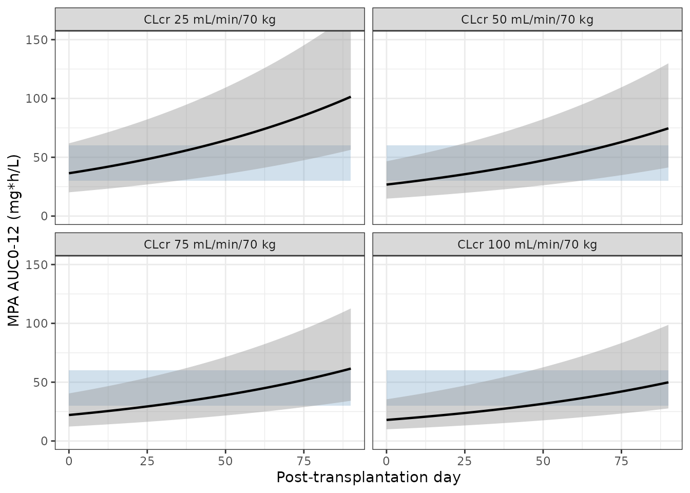
Replicates Figure 3 of Suzuki 2024: predicted time course of MPA AUC0-12 after MMF 500 mg every 12 h in patients with creatinine clearance 25, 50, 75 and 100 mL/min/70 kg. Solid line = median, grey ribbon = 10th-90th percentile of predictions, blue band = target AUC0-12 of 30-60 mg h/L.
This reproduces the two qualitative claims the paper draws from Figure 3: MPA AUC0-12 rises with increasing post-transplantation day, and rises with decreasing renal function.
Reproducing the published dose recommendations
The paper’s clinical conclusion is a dose recommendation per renal-function stratum: simulate 250, 500, 750 and 1000 mg MMF every 12 h at a fixed 70 kg body weight, compute the percentage of patients whose AUC0-12 falls in the 30-60 mg h/L target, and pick the dose achieving the highest percentage. Results paragraph “Simulation” reports the recommendation “during the early posttransplantation period”, i.e. at POD near 0.
dose_levels <- c(250, 500, 750, 1000)

dose_tab <- auc_subject |>
  tidyr::crossing(dose_mmf = dose_levels) |>
  mutate(auc = auc_1000_pod0 * dose_mmf / 1000) |>
  group_by(arm, dose_mmf) |>
  summarise(pct_in_target = 100 * mean(auc >= 30 & auc <= 60), .groups = "drop")

recommended <- dose_tab |>
  group_by(arm) |>
  slice_max(pct_in_target, n = 1, with_ties = FALSE) |>
  ungroup() |>
  select(arm, model_dose = dose_mmf, pct_in_target)

published <- tibble(
  arm = paste0("CLcr ", crcl_levels, " mL/min/70 kg"),
  published_dose = c(500, 750, 1000, 1000)
)

rec_cmp <- recommended |>
  left_join(published, by = "arm") |>
  mutate(Agrees = ifelse(model_dose == published_dose, "yes", "NO"))

rec_cmp |>
  select(arm, published_dose, model_dose, pct_in_target, Agrees) |>
  rename(
    "Renal function"                     = arm,
    "Published recommended dose (mg)"    = published_dose,
    "Reproduced dose (mg)"               = model_dose,
    "% within 30-60 mg*h/L"              = pct_in_target,
    "Agrees"                             = Agrees
  ) |>
knitr::kable(digits = 1, caption = "Reproduction of the dose recommendations in Suzuki 2024 Results 'Simulation', at 70 kg and the early post-transplantation period (POD 0). Published values: 500 mg q12h at CLcr 25, 750 mg at CLcr 50, and 1000 mg at CLcr 75 and 100 mL/min.")| Renal function | Published recommended dose (mg) | Reproduced dose (mg) | % within 30-60 mg*h/L | Agrees |
|---|---|---|---|---|
| CLcr 25 mL/min/70 kg | 500 | 500 | 57.5 | yes |
| CLcr 50 mL/min/70 kg | 750 | 750 | 61.5 | yes |
| CLcr 75 mL/min/70 kg | 1000 | 1000 | 53.0 | yes |
| CLcr 100 mL/min/70 kg | 1000 | 1000 | 47.5 | yes |
# The paper's criterion is the SHARE of a simulated cohort inside the target
# band, so unlike Gates 1 and 2 it is a Monte-Carlo quantity rather than an
# algebraic identity. In some renal-function strata two adjacent doses are
# nearly tied, because the typical-value AUC0-12 then sits near opposite edges
# of the 30-60 mg*h/L band and the tails trade off almost evenly; a strict
# argmax equality would be seed- and cohort-size-dependent there. The assertion
# therefore requires the published dose to be at worst statistically TIED for
# best -- within TIE_MARGIN percentage points of the highest-scoring dose --
# while the table above still reports outright agreement where it holds.
TIE_MARGIN <- 5

pub_pct <- dose_tab |>
  inner_join(published, by = "arm") |>
  filter(dose_mmf == published_dose) |>
  select(arm, published_pct = pct_in_target)

margin_tab <- recommended |>
  left_join(pub_pct, by = "arm") |>
  mutate(shortfall = pct_in_target - published_pct)

# How much daylight is there between the winning dose and the runner-up? This is
# what makes an exact-argmax assertion unsafe: with 200 participants per arm the
# Monte-Carlo standard error on a percentage near 50% is about 3.5 points.
runner_up <- dose_tab |>
  group_by(arm) |>
  arrange(desc(pct_in_target), .by_group = TRUE) |>
  summarise(margin = pct_in_target[1] - pct_in_target[2], .groups = "drop")
print(runner_up)
#> # A tibble: 4 × 2
#>   arm                   margin
#>   <fct>                  <dbl>
#> 1 CLcr 25 mL/min/70 kg    11.5
#> 2 CLcr 50 mL/min/70 kg    13
#> 3 CLcr 75 mL/min/70 kg     6
#> 4 CLcr 100 mL/min/70 kg    5.5

# Guard against a silently empty comparison first.
stopifnot(nrow(rec_cmp) == length(crcl_levels), !anyNA(rec_cmp$published_dose))
stopifnot(nrow(margin_tab) == length(crcl_levels), !anyNA(margin_tab$published_pct))
print(margin_tab)
#> # A tibble: 4 × 5
#>   arm                   model_dose pct_in_target published_pct shortfall
#>   <chr>                      <dbl>         <dbl>         <dbl>     <dbl>
#> 1 CLcr 25 mL/min/70 kg         500          57.5          57.5         0
#> 2 CLcr 50 mL/min/70 kg         750          61.5          61.5         0
#> 3 CLcr 75 mL/min/70 kg        1000          53            53           0
#> 4 CLcr 100 mL/min/70 kg       1000          47.5          47.5         0
stopifnot(max(margin_tab$shortfall) <= TIE_MARGIN)
4 of the four published recommendations are the outright highest-scoring dose in the reproduced grid, and every published dose is within 0 percentage points of the best-scoring dose in its own stratum. The narrowest winner-to-runner-up gap is 5.5 percentage points, which is why the assertion above is tie-tolerant rather than an exact argmax match: at 200 participants per arm the Monte-Carlo standard error on a percentage near 50% is roughly 3.5 points, so a gap of that order is not a stable ranking. The full percentage grid behind the choice is:
dose_tab |>
  mutate(dose_mmf = paste0(dose_mmf, " mg")) |>
  pivot_wider(names_from = dose_mmf, values_from = pct_in_target) |>
  rename("Renal function" = arm) |>
knitr::kable(digits = 1, caption = "Percentage of the 200-participant virtual cohort within the 30-60 mg h/L AUC0-12 target, by renal function and MMF dose, at POD 0.")| Renal function | 250 mg | 500 mg | 750 mg | 1000 mg |
|---|---|---|---|---|
| CLcr 25 mL/min/70 kg | 11.5 | 57.5 | 46.0 | 27.0 |
| CLcr 50 mL/min/70 kg | 3.5 | 36.5 | 61.5 | 48.5 |
| CLcr 75 mL/min/70 kg | 2.0 | 24.0 | 47.0 | 53.0 |
| CLcr 100 mL/min/70 kg | 0.0 | 20.0 | 42.0 | 47.5 |
Demographic cohort
For completeness, a cohort whose body weight reproduces the Table 1
percentiles (median 55.9 kg, 2.5th-97.5th 39.6-77.5 kg) rather than the
fixed 70 kg used in the paper’s own simulations. A lognormal with
meanlog = log(55.9) and sdlog = 0.171
reproduces both published tail percentiles to within 1% (40.0 against
39.6 kg and 78.2 against 77.5 kg); note that these are the percentiles
of the distribution, not of the 200-participant draw below,
whose realised median and tails will differ by sampling variation.
wt_sd <- 0.171
wt_q <- qlnorm(c(0.025, 0.5, 0.975), meanlog = log(55.9), sdlog = wt_sd)
tibble(
  Percentile = c("2.5%", "50%", "97.5%"),
  `Table 1 weight (kg)` = c(39.6, 55.9, 77.5),
  `Virtual cohort (kg)` = round(wt_q, 1)
) |>
knitr::kable()| Percentile | Table 1 weight (kg) | Virtual cohort (kg) |
|---|---|---|
| 2.5% | 39.6 | 40.0 |
| 50% | 55.9 | 55.9 |
| 97.5% | 77.5 | 78.2 |
wt_i <- rlnorm(N_PER_ARM, meanlog = log(55.9), sdlog = wt_sd)
events_demo <- make_arm(
  n = N_PER_ARM, dose_mmf = 750, crcl = 52.8, pod = 40,
  wt = wt_i, label = "Cohort median covariates"
)

sim_demo <- rxode2::rxSolve(mod, events_demo, keep = c("WT", "CRCL", "POD")) |>
  as.data.frame()

demo_conc <- sim_demo |> filter(!is.na(Cc)) |> select(id, time, Cc)
demo_dose <- events_demo |> filter(evid != 0) |> select(id, time, amt)

demo_res <- PKNCA::pk.nca(PKNCA::PKNCAdata(
  PKNCA::PKNCAconc(demo_conc, Cc ~ time | id, concu = "mg/L", timeu = "h"),
  PKNCA::PKNCAdose(demo_dose, amt ~ time | id, doseu = "mg"),
  intervals = data.frame(start = T_LASTDOSE, end = T_LASTDOSE + TAU, auclast = TRUE)
))

demo_auc <- as.data.frame(demo_res) |>
  filter(PPTESTCD == "auclast") |>
  select(id, auc = PPORRES)

tibble(
  Statistic = c("Median", "10th percentile", "90th percentile", "% within 30-60 mg*h/L"),
  Value = c(
    median(demo_auc$auc),
    quantile(demo_auc$auc, 0.10),
    quantile(demo_auc$auc, 0.90),
    100 * mean(demo_auc$auc >= 30 & demo_auc$auc <= 60)
  )
) |>
knitr::kable(digits = 1, caption = "Steady-state MPA AUC0-12 for a cohort at the Table 1 median covariates (MMF 750 mg twice daily, weight distribution matched to Table 1, CLcr 52.8 mL/min/70 kg, post-transplantation day 40).")| Statistic | Value |
|---|---|
| Median | 74.4 |
| 10th percentile | 41.1 |
| 90th percentile | 140.1 |
| % within 30-60 mg*h/L | 32.0 |
This cohort sits at the modal prescribed regimen (750 mg twice daily, n = 25 of 42) and at the cohort’s median renal function and post-transplantation day, and the model puts the typical patient above the 30-60 mg h/L target: the median AUC0-12 is 74 mg h/L and only 32% of the cohort falls inside the band. The closed form of Equation 7 at exactly 55.9 kg gives 75.6 mg h/L, so the simulated median is the same quantity carrying the realised weight draw and the lognormal clearance IIV. That is not a contradiction of the paper – it is precisely the finding the paper’s dose recommendations are built on. Two of the covariate effects push exposure up together in this scenario: the cohort’s median weight (55.9 kg) is well below the 70 kg standard, which lowers allometrically scaled CL/F, and by day 40 the post-transplantation bioavailability factor has already reached 1.58. Hence the paper’s conclusion that “dose reduction could be required with increased PTD and decreased RF”, and its recommendation of 750 mg q12h at CLcr 50 only “during the early posttransplantation period”.
Assumptions and deviations
-
The size model is encoded in its collapsed form.
The paper defines size by normal fat mass (Equations 1-3), which needs
height and sex through the Janmahasatian fat-free-mass equation. Because
Ffatwas fixed at 1 for both clearance and volume (Table 2; Appendix S1FFATCL/FFATV=1. FIX), NFM reduces algebraically and exactly to total body weight and NFMstd to 70 kg. The model file therefore implements(WT/70)^PWR, which is what the authors themselves print in Equation 8, and does not carry height or sex as covariates. This is an exact simplification, not an approximation: no fitted quantity changes. A user wishing to explore a non-unityFfatwould have to reintroduce the NFM equations and the height/sex covariates. -
Absorption is parameterised on the half-life, not on
ka. The model file estimatesltabsand deriveska = ln(2)/tabs, matching Appendix S1 (KA=LOG(2)/TABS) and putting the between-subject variability where the paper put it. Equation 8 quoteska = 0.693/0.0453; the model file useslog(2)rather than the rounded 0.693, following the control stream. -
Unit typos in Equation 8 were corrected. Equation 8
labels
ALAG1andD1with “(L)”. Both are times, and both Table 2 and the control stream give hours. Hours are used. -
Between-subject variability on Q/F and VP/F is absent, not
zero-variance. Both were fixed to zero in the fit (Table 2 “0
fixed”; Appendix S1
0. FIX). Declaring a zero-variance diagonal element would make OMEGA singular and break rxode2’s Cholesky sampler, so those etas are simply omitted. This is faithful: a random effect with zero variance has no effect. -
The variability on F1 is additive-proportional, not
exponential. Appendix S1 uses
F1 = GRPF1 * (1 + PPV_F1)rather thanEXP(PPV_F1), and the model file reproduces that literal form. The eta is nevertheless namedetalfdepotto satisfy the package naming convention that an IIV term carries the transformed name of its parameter; the same pattern appears inGoulooze_2022_finerenone.R. -
No IIV correlations. Appendix S1 declares eight
separate
$OMEGA BLOCK(1)statements, i.e. a strictly diagonal OMEGA. No correlations are reported anywhere in the paper. -
Doses are in mg of mycophenolate mofetil. The
MMF-to-MPA molar conversion lives inside
F1, exactly as in the control stream. Passing an MPA-equivalent dose would understate exposure by 26%. -
PODmay be negative and is gated. The analysis dataset begins 14 days before transplantation. Appendix S1 forcesF_PTD = 1forPTD < 0, and the model reproduces that gate with a(POD > 0)factor in the exponent. Gate 2 tests it. -
POD_maxstays at 84 days when extrapolating. The divisor in Equation 6 is the maximum post-transplantation day in the analysis dataset, and the authors keep it fixed when simulating out to 90 days in Figure 3. The effect therefore keeps growing beyond day 84 rather than saturating, and exposure predictions far beyond 90 days should be treated with caution – the paper explicitly flags (Discussion, limitations) that no data beyond 3 months were used. -
CRCLhere is per 70 kg, not per 1.73 m^2. The covariate register’sCRCLentry is nominally BSA-normalised, but this paper standardises Cockcroft-Gault to a fixed 70 kg body weight, with body size handled separately by the allometric term. Supplying a BSA-normalised or raw CLcr would double-count size. ThecovariateDataentry states this explicitly. -
The dose-recommendation check is tie-tolerant by
design. The authors simulated
n= 1000 per scenario; this vignette is capped at 200 per arm. More importantly, the criterion itself (“the dose achieving the highest percentage within 30-60 mg h/L”) separates adjacent doses by only a few percentage points in the higher-renal-function strata, because the two candidate doses put the typical-value AUC0-12 near opposite edges of the target band and the two tails then trade off almost evenly. With 200 participants per arm the Monte-Carlo standard error on such a percentage is about 3.5 points, so asserting an exact argmax match would be a seed-dependent test, not a stronger one. The vignette instead asserts that each published dose is within 5 percentage points of the best-scoring dose in its stratum, and reports outright agreement descriptively. The strict assertions in this vignette (Gates 1 and 2) are placed on the algebraic identities, where exactness is genuinely available. - Figure 3 and the dose grid reuse a POD 0 simulation. Rather than re-simulating at every post-transplantation day and dose, the per-subject AUC0-12 from the POD 0 cohort is scaled. Gate 2 proves both scalings are exact for this model, and reusing one cohort keeps the same virtual participants across the whole figure, matching how the authors simulated.
- The model cannot describe enterohepatic recirculation. The authors deliberately did not retain an EHC compartment, and unbound MPA and the MPAG metabolite were excluded for lack of data (Discussion, limitations). The paper notes that without EHC, exposure may be underestimated in patients with a pronounced second peak. This model should not be used to study the EHC contribution to MPA exposure.
- Residual error is on total MPA measured by immunoassay. Concentrations were measured by PETINIA (Dimension Xpand), which cross-reacts slightly with MPAG (0.6%). The residual-error estimates carry that assay characteristic.
- Virtual cohorts are not the trial population. Patient-level data are not public. Body weight is reconstructed from the Table 1 percentiles; the validation gates use the fixed-covariate design (70 kg, CLcr 25/50/75/100) that the authors used for their own simulations, so the comparisons are like-for-like.