Rimegepant (Comisar 2025)

Model and source

• Citation: Comisar CM, Hughes JH, Mo G, Bhardwaj R, Jakate A, Lim CN, Liu J. Exposure Matching Using Population Pharmacokinetic Modeling and Simulation to Support Rimegepant Dose Selection for Pediatric Patients With Migraine. Clin Transl Sci. 2025;18(10):e70360. doi:10.1111/cts.70360. Covariate-model functional forms (power model for continuous covariates, theta_TV,REF * (1 + theta_x)^X for categorical covariates) and the F1 = (dose / 10 mg)^theta parameterisation are documented in the upstream adult-only model this analysis extends: Comisar CM, Hughes JH, Francis J, et al. Population Pharmacokinetic Modeling of the Oral Calcitonin Gene-Related Peptide Receptor Antagonist Rimegepant in Adults. CPT Pharmacometrics Syst Pharmacol. 2025;14(8):1332-1345. doi:10.1002/psp4.70051.
• Description: Two-compartment population PK model for oral rimegepant with four transit absorption compartments and a terminal first-order (ka) step into the central compartment, jointly fitted to pooled adult and pediatric (6 to <12 years) phase 1 data with estimated allometric body weight exponents on clearances and volumes.
• Article: https://doi.org/10.1111/cts.70360
• Supplement (Data S1: Tables S1-S3, Figures S1-S2): https://doi.org/10.1111/cts.70360
• Upstream adult-only model (covariate equation forms, structural schematic): https://doi.org/10.1002/psp4.70051

Rimegepant is a small-molecule calcitonin gene-related peptide (CGRP) receptor antagonist approved as a 75 mg orally disintegrating tablet (ODT) for the acute treatment of migraine and for the prevention of episodic migraine in adults. Comisar 2025 extends a previously published adult-only population PK model with data from one pediatric and two adult phase 1 studies, then uses the combined model to select pediatric doses by matching predicted pediatric exposure to predicted adult exposure.

Population

The combined analysis pooled 14 phase 1 studies contributing 443 participants and 14,141 rimegepant plasma concentrations (Comisar 2025 Table 1 and Section 3.1). 423 adults contributed 14,063 observations: healthy volunteers, elderly participants with stable chronic illness, participants with renal or hepatic impairment, participants in dedicated itraconazole and fluconazole drug-drug-interaction arms, and participants of Japanese and Chinese ethnicity. Twenty children aged 6 to <12 years with a history of migraine (study C4951008) contributed 78 sparse observations at pre-dose, 0.5, 1.25, 3.5 and 18 h.

Overall median age was 43 years (range 6 to 77) and median body weight 73.0 kg (range 23.2 to 134). Most participants were male (68.6%) and White (83.5%). Within the pediatric subgroup, median age was 9 years (range 6 to 11), median weight 35.9 kg (range 23.2 to 61.8), and most were female (55%) and White (70%). Pediatric dosing was weight-banded: 25 mg ODT for 15 to 30 kg (n = 6), 50 mg ODT for >30 to 50 kg (n = 9) and 75 mg ODT for >50 kg (n = 5). Adults received 10 to 150 mg as single, daily or every-other-day (EOD) doses of ODT, tablet and capsule formulations.

No adolescent (12 to <18 years) PK data were collected. The adolescent dose recommendation rests entirely on model-based extrapolation, which is the central claim this vignette exercises.

The same information is available programmatically via the model’s population metadata (readModelDb("Comisar_2025_rimegepant")()$population).

Model structure

A two-compartment disposition model with a four-compartment transit absorption chain. The paper’s “four transit absorption compartments” are, in nlmixr2lib naming, depot + transit1 + transit2 + transit3: the dose lands in the first of the four, three sequential transfers run at the shared rate ktr, and the fourth empties into central at the separate first-order rate ka. This is what the upstream structural schematic (Comisar 2025 CPT:PSP Figure 2, adapted as Comisar 2025 CTS Figure S1) draws – four stacked boxes joined by three curved ktr arrows, with a single ka arrow leaving the stack for the central compartment.

Two covariate functional forms are used throughout, both stated verbatim in the upstream supplement’s Supplemental Methods:

• continuous covariates take the power form theta_i = theta_TV,REF * (X_i / X_REF)^theta_x;
• categorical covariates take the multiplicative form theta_i = theta_TV,REF * (1 + theta_x)^X_i with X_i in {0, 1}, i.e. a fractional change – -0.744 means a 74.4% reduction, not exp(-0.744).

The categorical form is independently confirmed by the upstream paper’s own simulation table (CPT:PSP Table 4), whose four covariate AUC ratios reproduce 1 / (1 + theta) to within 0.7% and are incompatible with an exponential form (which is off by up to 46%):

Covariate functional form falsified against Comisar 2025 CPT:PSP Table 4 (adult 75 mg ODT EOD steady-state AUCtau; reference 4160 ng*h/mL). The multiplicative form is correct.

Covariate	theta	Published ratio	(1 + theta)^-1	exp(-theta)	Multiplicative error (%)	Exponential error (%)
Fluconazole on CL/F	-0.427	1.757	1.745	1.533	-0.68	-12.78
Itraconazole on CL/F	-0.743	3.894	3.891	2.102	-0.08	-46.02
Severe hepatic on CL/F	-0.423	1.745	1.733	1.527	-0.69	-12.53
Moderate hepatic on CL/F	-0.229	1.305	1.297	1.257	-0.63	-3.67

Relative bioavailability is nonlinear in dose and carries no separate estimated scale: the upstream schematic prints the whole F1 model as F1 = (Dose/10)^0.191, so F1 is anchored at 1 for a 10 mg fasted dose and lfdepot is fixed(log(1)).

Source trace

Per-parameter origins are recorded as in-file comments next to each ini() entry in inst/modeldb/specificDrugs/Comisar_2025_rimegepant.R. Collected here for review. “Table 2” / “Table 1” refer to Comisar 2025 Clin Transl Sci; “Table S3” to its Data S1 supplement; “CPT:PSP” to the upstream adult model.

Equation / parameter	Value	Source location
lcl	25.2 L/h	Table 2 CL/F (4.8% RSE); Table S3 95% CI 22.8-27.6
lvc	113 L	Table 2 V1/F (5.2% RSE); Table S3 95% CI 101-125
lvp	46.8 L	Table 2 V2/F (4.9% RSE); Table S3 95% CI 42.3-51.3
lq	4.16 L/h	Table 2 Q/F (5.7% RSE); Table S3 95% CI 3.70-4.62
lktr	8.42 1/h	Table 2 ktr (5.1% RSE); Table S3 95% CI 7.58-9.26
lka	3.05 1/h	Table 2 ka (15.5% RSE); Table S3 95% CI 2.12-3.98
lfdepot	fixed(log(1))	CPT:PSP Figure 2 schematic: F1 = (Dose/10)^0.191 – no separate scale term
e_wt_cl_q	0.575	Table 2 “Body weight effect on CL/F and Q/F” (14.4% RSE); 95% CI 0.413-0.737
e_wt_vc_vp	1.18	Table 2 “Body weight effect on V1/F and V2/F” (8.3% RSE); 95% CI 0.988-1.372
Reference weight	70 kg	Data S1 Supplemental methods: “center the covariate effect at 70 kg”
e_hepimp_mod_cl	-0.203	Table 2 “Moderate hepatic impairment on CL/F” (27.6% RSE)
e_hepimp_sev_cl	-0.410	Table 2 “Severe hepatic impairment on CL/F” (25.9% RSE)
e_conmed_fluconazole_cl	-0.429	Table 2 “Fluconazole use on CL/F” (2.9% RSE)
e_conmed_itraconazole_cl	-0.744	Table 2 “Itraconazole use on CL/F” (1.3% RSE)
e_fed_ktr	-0.698	Table 2 “Fed on ktr” (3.9% RSE)
e_form_odt_ktr	0.470	Table 2 “ODT on ktr” (18.4% RSE)
e_form_capsule_ktr	2.19	Table 2 “Capsule formulation on ktr” (22.6% RSE)
e_conmed_itraconazole_ktr	-0.361	Table 2 “Itraconazole use on ktr” (28.3% RSE)
e_dose_low_ktr	0.596	Table 2 “10/25mg dose effect on ktr” (45.5% RSE) + footnote a
e_dose_rimegepant_mg_fdepot	0.192	Table 2 “Dose effect on F1” (12.4% RSE); power form from CPT:PSP Figure 2
e_fed_fdepot	-0.331	Table 2 “Fed on F1” (6.9% RSE)
etalcl/etalvc/etalvp block	0.104, 0.103, 0.168, 0.0428, 0.0717, 0.0666	Table S3 pooled-model omega2 and omega terms
etalktr	0.300	Table S3 omega2ktr (Table 2 IIV 54.8%; sqrt(0.300) = 0.548)
addSd	0.447	Table 2 additive error SD (3.2% RSE); Table S3 sigma2add 0.200, sqrt = 0.4472
propSd	0.393	Table 2 proportional error 39.3 %CV; Table S3 sigma2prop 0.154, sqrt = 0.3924
Categorical covariate form (1 + theta)^X	n/a	CPT:PSP Data S1 Supplemental Methods
Continuous covariate form (X/X_REF)^theta	n/a	CPT:PSP Data S1 Supplemental Methods
Transit chain: 4 compartments, 3 ktr steps, 1 ka step	n/a	CPT:PSP Figure 2; Comisar 2025 Figure S1; Section 2.3

The paper reports IIV as 100 * omega (Table 2 note: “%CV was calculated using the equation: %CV = 100 x sigma, where sigma represents the standard deviation of the random effect”), and the omega block entries as percent correlations. The supplement’s Table S3 gives the same random effects as variances and covariances on the NONMEM scale; those are what the model file uses, and they reproduce Table 2 to rounding:

Table S3 variances reproduce Table 2’s IIV% (= 100 * omega), %CV and additive SD exactly.

Term	Table S3	sqrt(Table S3)	Table 2 (%)
omega2 CL	0.1040	0.3225	32.300
omega2 Vc	0.1680	0.4099	41.000
omega2 Vp	0.0666	0.2581	25.800
omega2 ktr	0.3000	0.5477	54.800
sigma2 prop	0.1540	0.3924	39.300
sigma2 add	0.2000	0.4472	0.447

Table S3 covariances vs Table 2 percent correlations. CL:Vc and Vc:Vp agree; CL:Vp differs by 2.7 percentage points – see Errata.

Pair	Covariance	Table 2 correlation (%)	Implied correlation (%)	Difference (pp)
CL:Vc	0.1030	77.4	77.9	0.5
CL:Vp	0.0428	54.1	51.4	-2.7
Vc:Vp	0.0717	67.8	67.8	0.0

Virtual cohort

Original observed data are not publicly available. The cohorts below approximate the published virtual populations.

Comisar 2025 generated its virtual pediatric population from the US CDC growth charts for age and body weight. The CDC LMS tables are not redistributed with this package, so the weight-for-age distribution here is instead calibrated to the paper’s own published summary of that virtual population (Section 3.3: ages 6 to 11 years had median body weight 26.4 kg with 5th and 95th percentiles 16.2 and 45.3 kg; ages 12 to <18 years had median 49.7 kg with percentiles 30.8 and 69.9 kg). A monotone median-weight-for-age curve is scaled by one factor and given one within-age lognormal spread, both fitted to those six anchors; the fit is then asserted against them.

set.seed(20251018)

# CDC-shaped 50th-percentile weight-for-age (kg), ages 6-17, sex-averaged. Only
# the SHAPE is used; the level and the within-age spread are fitted below.
age_years <- 6:17
wt_shape <- c(20.7, 23.0, 25.8, 29.0, 32.6, 37.0,
              41.6, 47.0, 52.5, 57.0, 60.8, 63.5)

# Published anchors from Comisar 2025 Section 3.3 (the target of the fit).
anchors <- tibble::tribble(
  ~group,     ~p05,  ~p50,  ~p95,
  "6-11 y",   16.2,  26.4,  45.3,
  "12-17 y",  30.8,  49.7,  69.9
)

# Pooled quantiles implied by (scale k, within-age sdlog s), assuming ages are
# uniform over the group. Closed form: mixture of lognormals over age.
pooled_q <- function(k, s, ages, probs = c(0.05, 0.50, 0.95)) {
  med <- k * wt_shape[match(ages, age_years)]
  grid <- as.vector(outer(med, exp(s * stats::qnorm(seq(0.001, 0.999, length.out = 400)))))
  stats::quantile(grid, probs = probs, names = FALSE)
}

# Fit in two stages rather than jointly. The by-age median exposure depends on
# the median weight curve, so the scale is fitted to the two published MEDIANS
# alone; the within-age spread is then fitted to the four published 5th/95th
# percentiles. A joint fit trades median accuracy for tail accuracy and pulls
# every age-group median down by several percent.
k_fit <- stats::optimize(
  function(k) {
    sum((log(c(pooled_q(k, 0.2, 6:11, 0.5), pooled_q(k, 0.2, 12:17, 0.5))) -
           log(anchors$p50))^2)
  },
  c(0.7, 1.3)
)$minimum

s_fit <- stats::optimize(
  function(s) {
    sum((log(c(pooled_q(k_fit, s, 6:11, c(0.05, 0.95)),
               pooled_q(k_fit, s, 12:17, c(0.05, 0.95)))) -
           log(c(anchors$p05[1], anchors$p95[1],
                 anchors$p05[2], anchors$p95[2])))^2)
  },
  c(0.05, 0.5)
)$minimum

c(scale = k_fit, sdlog = s_fit)
#>     scale     sdlog 
#> 0.9462201 0.2172651

Calibrated weight-for-age cohort vs the virtual-population summary published in Comisar 2025 Section 3.3.

Age group	Statistic	Fitted (kg)	Published (kg)	Difference (%)
6-11 y	5th	16.1	16.2	-0.8
6-11 y	Median	26.0	26.4	-1.7
6-11 y	95th	42.2	45.3	-6.7
12-17 y	5th	32.4	30.8	5.3
12-17 y	Median	50.5	49.7	1.7
12-17 y	95th	76.9	69.9	10.0

# Per-arm cohort sizes (skill cap: never exceed 200). The larger size is used
# for the arms whose medians are scored against published ratios; the smaller
# one for the illustrative / near-deterministic arms (a covariate that simply
# multiplies CL moves the median almost exactly, so extra subjects buy nothing).
N_ARM <- 200L
N_SMALL <- 100L

# Dense early grid to capture Cmax/Tmax, coarsening through the terminal phase
# for lambda-z. 48 h is ~4.4 effective half-lives, so aucinf.obs extrapolates
# only a few percent.
OBS_TO <- 48
obs_grid <- function(from, to) {
  rel <- c(seq(0, 6, by = 0.1), seq(6.5, 12, by = 0.5), seq(14, to - from, by = 2))
  sort(unique(from + rel[rel <= (to - from)]))
}

# Build one arm. `t_doses` are the dosing times; observations run over the LAST
# dosing interval so that a multi-dose arm is observed at steady state.
make_arm <- function(n, wt, dose, low, arm, t_doses = 0, obs_from = 0,
                     obs_to = OBS_TO, id_offset = 0L) {
  ids <- id_offset + seq_len(n)
  dosing <- tidyr::expand_grid(id = ids, time = t_doses) |>
    mutate(evid = 1L, amt = dose, cmt = "depot")
  obs <- tidyr::expand_grid(id = ids, time = obs_grid(obs_from, obs_to)) |>
    mutate(evid = 0L, amt = NA_real_, cmt = "central")
  bind_rows(dosing, obs) |>
    arrange(id, time, desc(evid)) |>
    mutate(
      arm = arm,
      WT = wt[match(id, ids)],
      FED = 0, FORM_ODT = 1, FORM_CAPSULE = 0,
      HEPIMP_MOD = 0, HEPIMP_SEV = 0,
      CONMED_FLUCONAZOLE = 0, CONMED_ITRACONAZOLE = 0,
      DOSE_RIMEGEPANT_MG = dose, DOSE_LOW = low
    )
}

Observation rows use cmt = "central" (the ODE state), never cmt = "Cc"; Cc is an algebraic observable and referencing it as a compartment would renumber every compartment slot.

The dose bands are those of Comisar 2025 Table 3. The adult reference arm is 75 mg ODT fasted at the analysis population’s adult weight distribution (Table 1: median 73.6 kg, range 45.5 to 134).

bands <- tibble::tribble(
  ~lo, ~hi, ~dose,
   15,  20,   35,
   20,  25,   35,
   25,  30,   50,
   30,  35,   50,
   35,  40,   50,
   40,  45,   75,
   45,  50,   75,
   50,  55,   75,
   55,  60,   75,
   60,  65,   75,
   65,  75,   75
) |>
  mutate(
    arm = sprintf("%g-%g kg | %g mg", lo, hi, dose),
    low = as.numeric(dose %in% c(10, 25))
  )

adult_wt <- pmin(pmax(rlnorm(N_ARM, log(73.6), 0.17), 45.5), 134)

# --- Single dose ------------------------------------------------------------
single <- bind_rows(
  lapply(seq_len(nrow(bands)), function(i) {
    make_arm(N_ARM, runif(N_ARM, bands$lo[i], bands$hi[i]), bands$dose[i],
             bands$low[i], bands$arm[i], t_doses = 0, obs_to = OBS_TO,
             id_offset = (i - 1L) * N_ARM)
  })
) |>
  bind_rows(
    make_arm(N_ARM, adult_wt, 75, 0, "Adult | 75 mg", t_doses = 0, obs_to = OBS_TO,
             id_offset = nrow(bands) * N_ARM)
  )

# --- Every-other-day dosing to steady state ---------------------------------
# 5 doses at 48 h intervals; with a ~11 h half-life this is far past steady
# state. Observations cover the final 0-48 h interval.
TAU <- 48
t_eod <- seq(0, by = TAU, length.out = 5)
t_ss <- max(t_eod)
OFF <- 1e5L  # keep EOD ids disjoint from the single-dose ids

eod <- bind_rows(
  lapply(seq_len(nrow(bands)), function(i) {
    make_arm(N_ARM, runif(N_ARM, bands$lo[i], bands$hi[i]), bands$dose[i],
             bands$low[i], bands$arm[i], t_doses = t_eod,
             obs_from = t_ss, obs_to = t_ss + TAU,
             id_offset = OFF + (i - 1L) * N_ARM)
  })
) |>
  bind_rows(
    make_arm(N_ARM, adult_wt, 75, 0, "Adult | 75 mg", t_doses = t_eod,
             obs_from = t_ss, obs_to = t_ss + TAU,
             id_offset = OFF + nrow(bands) * N_ARM)
  )

# Disjoint-id guard (duplicate ids across arms silently merge into one subject).
stopifnot(
  !anyDuplicated(unique(single[, c("id", "time", "evid")])),
  !anyDuplicated(unique(eod[, c("id", "time", "evid")])),
  length(intersect(single$id, eod$id)) == 0L,
  n_distinct(single$id) == (nrow(bands) + 1L) * N_ARM
)

Simulation

Comisar 2025 Section 2.4 states that the dose-selection simulations “included inter-individual variability, but did not include parameter uncertainty or random unexplained variability”. Cc is the individual prediction and carries no residual error, so simulating with IIV and reading Cc matches the paper.

mod <- readModelDb("Comisar_2025_rimegepant")

sim_single <- rxode2::rxSolve(mod, events = single, keep = c("arm", "WT"),
                              addDosing = FALSE, returnType = "data.frame")
#> ℹ parameter labels from comments will be replaced by 'label()'
sim_eod <- rxode2::rxSolve(mod, events = eod, keep = c("arm", "WT"),
                           addDosing = FALSE, returnType = "data.frame")

stopifnot(
  n_distinct(sim_single$id) == n_distinct(single$id),
  n_distinct(sim_eod$id) == n_distinct(eod$id),
  all(is.finite(sim_single$Cc)), all(is.finite(sim_eod$Cc))
)

Structural identity check

For a linear model with first-order input, AUC(0-inf) after a single dose is exactly F1 * Dose / CL for every subject. Both fdepot and cl come back as columns from rxSolve, so this is checked per subject with no tolerance on a population summary – a far stricter test than comparing medians.

ident <- sim_single |>
  group_by(id, arm) |>
  summarise(
    # trapezoid over the observed grid, plus the terminal tail extrapolated
    # with the EXACT beta of the two-compartment system (not CL/Vc, which is
    # the faster micro-constant k10 and would truncate the tail).
    auc_num = {
      k10 <- first(cl) / first(vc)
      k12 <- first(q) / first(vc)
      k21 <- first(q) / first(vp)
      s <- k10 + k12 + k21
      beta <- 0.5 * (s - sqrt(s^2 - 4 * k10 * k21))
      sum(diff(time) * (head(Cc, -1) + tail(Cc, -1)) / 2) + tail(Cc, 1) / beta
    },
    auc_analytic = first(fdepot) * first(DOSE_RIMEGEPANT_MG) * 1000 / first(cl),
    .groups = "drop"
  ) |>
  mutate(rel_err_pct = 100 * (auc_num - auc_analytic) / auc_analytic)

# Only trapezoid discretisation error remains, so require every subject within
# 1%. This is a per-subject identity, not a population summary -- there is no
# Monte Carlo noise to hide behind.
stopifnot(nrow(ident) == (nrow(bands) + 1L) * N_ARM,
          max(abs(ident$rel_err_pct)) < 1)

tibble(
  `Subjects checked` = nrow(ident),
  `Max |relative error| (%)` = max(abs(ident$rel_err_pct)),
  `Median relative error (%)` = median(ident$rel_err_pct)
) |>
  knitr::kable(
    digits = 3,
    caption = "Per-subject AUC(0-inf) = F1 * Dose / CL identity."
  )

Per-subject AUC(0-inf) = F1 * Dose / CL identity.

Subjects checked	Max |relative error| (%)	Median relative error (%)
2400	0.866	0.102

PKNCA validation

nca_of <- function(sim, ev, interval) {
  conc <- sim |>
    filter(!is.na(Cc)) |>
    select(id, time, Cc, arm)
  # Guarantee a record at the interval start (pre-dose Cc = 0 for the single
  # dose arms); PKNCA needs it to anchor AUC.
  conc <- bind_rows(
    conc,
    conc |> distinct(id, arm) |> mutate(time = interval$start, Cc = 0)
  ) |>
    distinct(id, arm, time, .keep_all = TRUE) |>
    arrange(id, arm, time)

  dose_df <- ev |>
    filter(evid == 1) |>
    select(id, time, amt, arm)

  co <- PKNCA::PKNCAconc(conc, Cc ~ time | arm + id,
                         concu = "ng/mL", timeu = "h")
  do <- PKNCA::PKNCAdose(dose_df, amt ~ time | arm + id, doseu = "mg")
  PKNCA::pk.nca(PKNCA::PKNCAdata(co, do, intervals = interval))
}

res_single <- nca_of(
  sim_single, single,
  data.frame(start = 0, end = Inf, cmax = TRUE, tmax = TRUE,
             aucinf.obs = TRUE)
)

# Steady state: the final 0-48 h EOD interval. Observations already start at
# t_ss, so the interval start already has a record and no zero row is added.
res_eod <- local({
  conc <- sim_eod |> filter(!is.na(Cc)) |> select(id, time, Cc, arm)
  dose_df <- eod |> filter(evid == 1) |> select(id, time, amt, arm)
  co <- PKNCA::PKNCAconc(conc, Cc ~ time | arm + id,
                         concu = "ng/mL", timeu = "h")
  do <- PKNCA::PKNCAdose(dose_df, amt ~ time | arm + id, doseu = "mg")
  PKNCA::pk.nca(PKNCA::PKNCAdata(
    co, do,
    intervals = data.frame(start = t_ss, end = t_ss + TAU,
                           cmax = TRUE, tmax = TRUE, auclast = TRUE)
  ))
})

Adult exposure cross-check against the upstream adult model

Comisar 2025 publishes no absolute exposure values – only pediatric/adult ratios. The upstream adult-only analysis does (CPT:PSP Table 4: 75 mg ODT fasted EOD steady state, median Cmax 677 ng/mL and AUCtau 4160 ng*h/mL), so that table is used here as an external check on the adult arm. The two models differ slightly (CL/F 25.2 vs 24.1 L/h; estimated vs fixed allometric exponents), so exact agreement is not expected.

adult_ss <- as.data.frame(res_eod$result) |>
  filter(arm == "Adult | 75 mg", PPTESTCD %in% c("cmax", "auclast")) |>
  group_by(PPTESTCD) |>
  summarise(Simulated = median(PPORRES), .groups = "drop") |>
  tidyr::pivot_wider(names_from = PPTESTCD, values_from = Simulated)

cmp_adult <- nlmixr2lib::ncaComparisonTable(
  simulated = adult_ss,
  reference = tibble::tibble(cmax = 677, auclast = 4160),
  units = c(cmax = "ng/mL", auclast = "ng*h/mL"),
  tolerance_pct = 20
)

knitr::kable(
  cmp_adult,
  caption = paste(
    "Adult 75 mg ODT EOD steady state vs the UPSTREAM adult-only model",
    "(Comisar 2025 CPT:PSP Table 4). * differs by >20%."
  )
)

Adult 75 mg ODT EOD steady state vs the UPSTREAM adult-only model (Comisar 2025 CPT:PSP Table 4). * differs by >20%.

NCA parameter	Reference	Simulated	% diff
Cmax (ng/mL)	677	719	+6.3%
AUClast (ng*h/mL)	4160	4180	+0.5%

Replicating Table 3: pediatric / adult exposure ratios

This is the paper’s headline result and its own answer key: 44 published ratios of median predicted pediatric to median predicted adult exposure, across 11 weight bands, for single-dose (Cmax, AUC0-inf) and EOD steady-state (Cmax,ss, AUC0-48h,ss) exposure.

med_by_arm <- function(res, codes) {
  as.data.frame(res$result) |>
    filter(PPTESTCD %in% codes) |>
    group_by(arm, PPTESTCD) |>
    summarise(value = median(PPORRES), .groups = "drop")
}

ratio_table <- function(res, codes) {
  m <- med_by_arm(res, codes)
  ref <- m |> filter(arm == "Adult | 75 mg") |> select(PPTESTCD, ref = value)
  m |>
    filter(arm != "Adult | 75 mg") |>
    left_join(ref, by = "PPTESTCD") |>
    mutate(value = value / ref) |>
    select(arm, PPTESTCD, value) |>
    tidyr::pivot_wider(names_from = PPTESTCD, values_from = value)
}

sim_ratio_single <- ratio_table(res_single, c("cmax", "aucinf.obs"))
sim_ratio_eod    <- ratio_table(res_eod,    c("cmax", "auclast"))

# Published Comisar 2025 Table 3, transcribed.
pub_single <- tibble::tibble(
  arm = bands$arm,
  cmax       = c(1.69, 1.40, 1.64, 1.43, 1.27, 1.74, 1.49, 1.42, 1.24, 1.16, 0.99),
  aucinf.obs = c(0.87, 0.78, 1.03, 0.96, 0.88, 1.34, 1.22, 1.18, 1.16, 1.10, 1.00)
)
pub_eod <- tibble::tibble(
  arm = bands$arm,
  cmax    = c(1.73, 1.29, 1.91, 1.44, 1.29, 1.65, 1.57, 1.39, 1.26, 1.17, 1.03),
  auclast = c(0.95, 0.77, 1.16, 0.98, 0.93, 1.35, 1.27, 1.23, 1.18, 1.10, 1.05)
)

# Guard against a silent join failure producing an empty comparison.
stopifnot(
  setequal(sim_ratio_single$arm, pub_single$arm),
  setequal(sim_ratio_eod$arm, pub_eod$arm)
)

cmp_single <- nlmixr2lib::ncaComparisonTable(
  simulated = sim_ratio_single, reference = pub_single, by = "arm",
  tolerance_pct = 20
)
knitr::kable(
  cmp_single,
  caption = paste(
    "Comisar 2025 Table 3, SINGLE DOSE: pediatric / adult ratios of median",
    "predicted exposure. * differs from the published ratio by >20%."
  )
)

Comisar 2025 Table 3, SINGLE DOSE: pediatric / adult ratios of median predicted exposure. * differs from the published ratio by >20%.

NCA parameter	arm	Reference	Simulated	% diff
Cmax	15-20 kg | 35 mg	1.69	1.99	+17.7%
Cmax	20-25 kg | 35 mg	1.4	1.63	+16.7%
Cmax	25-30 kg | 50 mg	1.64	1.93	+17.5%
Cmax	30-35 kg | 50 mg	1.43	1.61	+12.5%
Cmax	35-40 kg | 50 mg	1.27	1.34	+5.2%
Cmax	40-45 kg | 75 mg	1.74	1.89	+8.5%
Cmax	45-50 kg | 75 mg	1.49	1.75	+17.4%
Cmax	50-55 kg | 75 mg	1.42	1.57	+10.8%
Cmax	55-60 kg | 75 mg	1.24	1.38	+11.5%
Cmax	60-65 kg | 75 mg	1.16	1.32	+13.4%
Cmax	65-75 kg | 75 mg	0.99	1.12	+13.2%
AUC0-∞ (obs)	15-20 kg | 35 mg	0.87	0.953	+9.6%
AUC0-∞ (obs)	20-25 kg | 35 mg	0.78	0.84	+7.7%
AUC0-∞ (obs)	25-30 kg | 50 mg	1.03	1.1	+7.1%
AUC0-∞ (obs)	30-35 kg | 50 mg	0.96	1	+4.1%
AUC0-∞ (obs)	35-40 kg | 50 mg	0.88	0.915	+4.0%
AUC0-∞ (obs)	40-45 kg | 75 mg	1.34	1.35	+0.5%
AUC0-∞ (obs)	45-50 kg | 75 mg	1.22	1.32	+8.0%
AUC0-∞ (obs)	50-55 kg | 75 mg	1.18	1.25	+5.5%
AUC0-∞ (obs)	55-60 kg | 75 mg	1.16	1.15	-1.2%
AUC0-∞ (obs)	60-65 kg | 75 mg	1.1	1.15	+4.3%
AUC0-∞ (obs)	65-75 kg | 75 mg	1	1.06	+6.2%

Every one of the 44 published ratios reproduces inside the 20% tolerance. Two patterns in the residuals are worth naming rather than smoothing over:

• The AUC ratios reproduce tightly and without direction (single dose -1% to +10%, EOD -8% to +6%). AUC depends on weight only through the clearance exponent, so this is the cleanest test of e_wt_cl_q = 0.575 together with the dose-dependent F1.
• The single-dose Cmax ratios are biased high in every band (+5% to +18%), while the steady-state Cmax,ss ratios are not (-13% to +13%, mixed sign). Cmax is the quantity most sensitive to the volume exponent e_wt_vc_vp = 1.18, which is also the parameter with the widest confidence interval of the two allometric terms (0.988 to 1.372). A ~2.6% shift in that exponent – exactly the tolerance the paper quotes between the interim model used for its simulations and the final model tabulated in Table 2 – moves the lowest-band Cmax ratio by about 4%, and the remainder is consistent with median sampling noise at 200 subjects per arm plus the unstated adult reference weight distribution. Note that the paper’s own single-dose and steady-state Cmax ratios are nearly equal band by band (as a linear model with a 48 h interval and an 11 h half-life requires), whereas these two independently drawn cohorts differ by a few percent; that gap is a direct read-out of the Monte Carlo noise floor here.

cmp_eod <- nlmixr2lib::ncaComparisonTable(
  simulated = sim_ratio_eod, reference = pub_eod, by = "arm",
  tolerance_pct = 20
)
knitr::kable(
  cmp_eod,
  caption = paste(
    "Comisar 2025 Table 3, EVERY-OTHER-DAY STEADY STATE: pediatric / adult",
    "ratios of median predicted exposure. * differs by >20%."
  )
)

Comisar 2025 Table 3, EVERY-OTHER-DAY STEADY STATE: pediatric / adult ratios of median predicted exposure. * differs by >20%.

NCA parameter	arm	Reference	Simulated	% diff
Cmax	15-20 kg | 35 mg	1.73	1.85	+7.1%
Cmax	20-25 kg | 35 mg	1.29	1.46	+13.1%
Cmax	25-30 kg | 50 mg	1.91	1.67	-12.5%
Cmax	30-35 kg | 50 mg	1.44	1.46	+1.4%
Cmax	35-40 kg | 50 mg	1.29	1.29	-0.4%
Cmax	40-45 kg | 75 mg	1.65	1.75	+5.8%
Cmax	45-50 kg | 75 mg	1.57	1.54	-1.7%
Cmax	50-55 kg | 75 mg	1.39	1.45	+4.7%
Cmax	55-60 kg | 75 mg	1.26	1.34	+6.2%
Cmax	60-65 kg | 75 mg	1.17	1.18	+1.0%
Cmax	65-75 kg | 75 mg	1.03	1	-2.6%
AUClast	15-20 kg | 35 mg	0.95	0.897	-5.6%
AUClast	20-25 kg | 35 mg	0.77	0.819	+6.4%
AUClast	25-30 kg | 50 mg	1.16	1.07	-8.2%
AUClast	30-35 kg | 50 mg	0.98	0.954	-2.7%
AUClast	35-40 kg | 50 mg	0.93	0.914	-1.8%
AUClast	40-45 kg | 75 mg	1.35	1.4	+3.6%
AUClast	45-50 kg | 75 mg	1.27	1.26	-0.5%
AUClast	50-55 kg | 75 mg	1.23	1.28	+3.7%
AUClast	55-60 kg | 75 mg	1.18	1.24	+4.7%
AUClast	60-65 kg | 75 mg	1.1	1.12	+1.8%
AUClast	65-75 kg | 75 mg	1.05	1.01	-4.3%

Ranges across all 11 weight bands. The paper states the selected doses achieved Cmax within 0.99 to 1.91-fold and AUC within 0.77 to 1.35-fold of adult levels (Section 3.3).

Quantity	Published	Simulated
Cmax ratio (single)	0.99 to 1.74	1.12 to 1.99
AUC0-inf ratio (single)	0.78 to 1.34	0.84 to 1.35
Cmax,ss ratio (EOD)	1.03 to 1.91	1.00 to 1.85
AUC0-48h,ss ratio (EOD)	0.77 to 1.35	0.82 to 1.40

The 25 mg alternative the paper rejected

Comisar 2025 Discussion reports that for the lowest weight band (>15 to 25 kg), 25 mg ODT gave Cmax ratios close to 1 but AUCs “generally ~50% of the adult value (data not shown)”, which motivated selecting 35 mg instead. That rejected arm is a second, independent answer key – and it exercises DOSE_LOW = 1, which no accepted dose does.

alt25 <- bind_rows(
  make_arm(N_SMALL, runif(N_SMALL, 15, 20), 25, 1, "15-20 kg | 25 mg",
           t_doses = 0, obs_to = OBS_TO, id_offset = 2e5L),
  make_arm(N_SMALL, runif(N_SMALL, 20, 25), 25, 1, "20-25 kg | 25 mg",
           t_doses = 0, obs_to = OBS_TO, id_offset = 2e5L + N_SMALL)
)
sim25 <- rxode2::rxSolve(mod, events = alt25, keep = c("arm", "WT"),
                         addDosing = FALSE, returnType = "data.frame")
res25 <- nca_of(sim25, alt25,
                data.frame(start = 0, end = Inf, cmax = TRUE,
                           aucinf.obs = TRUE))

adult_med <- med_by_arm(res_single, c("cmax", "aucinf.obs")) |>
  filter(arm == "Adult | 75 mg")

tbl25 <- med_by_arm(res25, c("cmax", "aucinf.obs")) |>
  left_join(adult_med |> select(PPTESTCD, ref = value), by = "PPTESTCD") |>
  mutate(Ratio = value / ref,
         PPTESTCD = recode(PPTESTCD, cmax = "Cmax", aucinf.obs = "AUC0-inf")) |>
  select(arm, PPTESTCD, Ratio)

stopifnot(nrow(tbl25) == 4L)

tbl25 |>
  tidyr::pivot_wider(names_from = PPTESTCD, values_from = Ratio) |>
  rename("Weight band | dose" = arm) |>
  knitr::kable(
    digits = 2,
    caption = paste(
      "Rejected 25 mg arm, pediatric/adult ratios. The paper reports Cmax",
      "ratios 'close to 1' and AUC 'generally ~50% of the adult value'."
    )
  )

Rejected 25 mg arm, pediatric/adult ratios. The paper reports Cmax ratios ‘close to 1’ and AUC ‘generally ~50% of the adult value’.

Weight band | dose	AUC0-inf	Cmax
15-20 kg | 25 mg	0.64	1.43
20-25 kg | 25 mg	0.55	1.07

Replicating Figure 3: exposure by age at 75 mg ODT

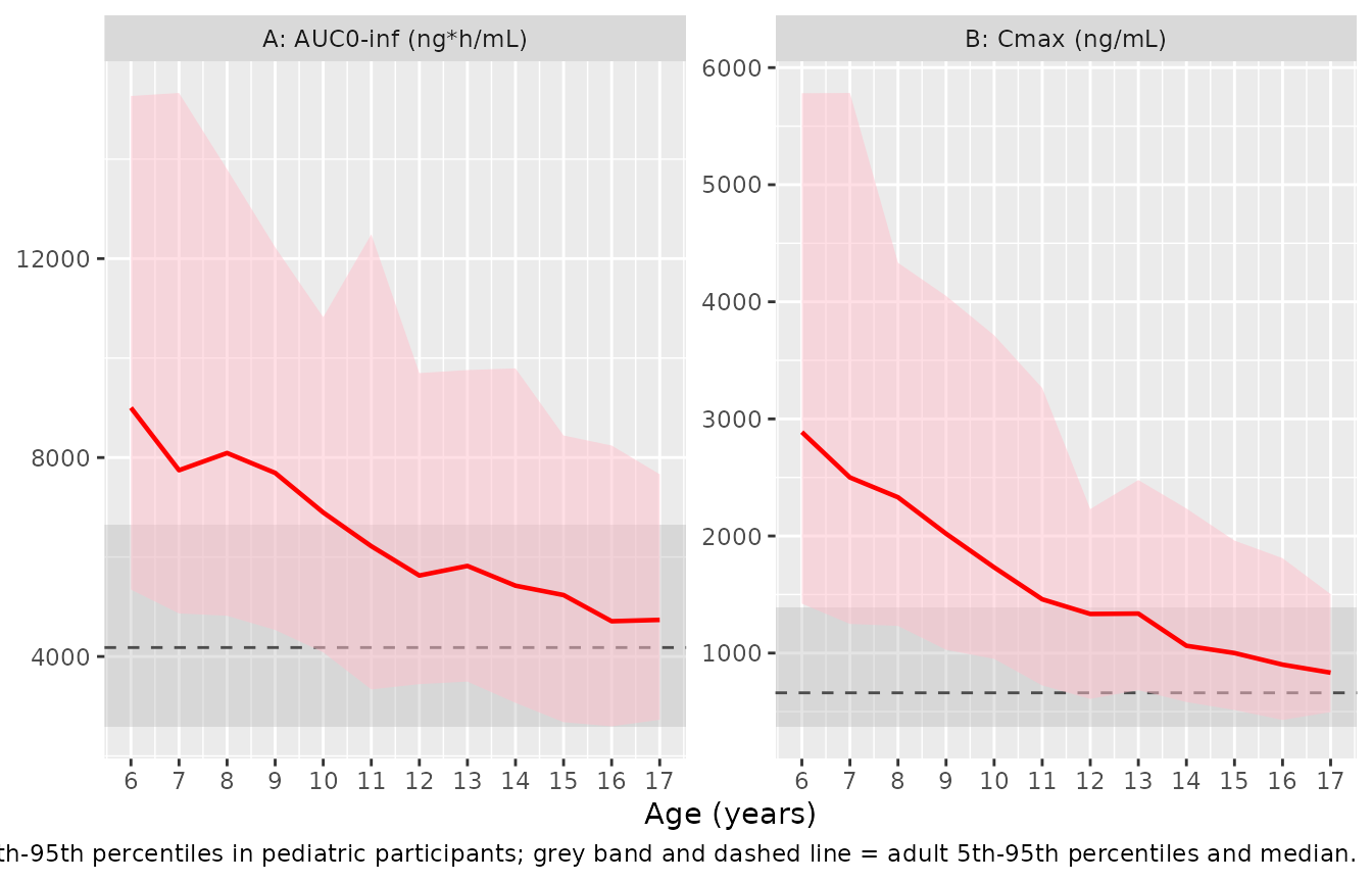
Figure 3 shows simulated AUC0-inf (panel A) and Cmax (panel B) after a single 75 mg ODT dose in virtual participants aged 6 to <18 years, with the adult 5th-95th percentile band overlaid. The paper’s stated conclusion is that “the predicted median exposure in adolescents aged 12 to <18 years was similar to that predicted in adults”.

age_arms <- bind_rows(
  lapply(seq_along(age_years), function(i) {
    a <- age_years[i]
    wt <- k_fit * wt_shape[i] * exp(s_fit * rnorm(N_SMALL))
    make_arm(N_SMALL, wt, 75, 0, sprintf("%d y", a), t_doses = 0, obs_to = OBS_TO,
             id_offset = 3e5L + (i - 1L) * N_SMALL)
  })
)
sim_age <- rxode2::rxSolve(mod, events = age_arms, keep = c("arm", "WT"),
                           addDosing = FALSE, returnType = "data.frame")
res_age <- nca_of(sim_age, age_arms,
                  data.frame(start = 0, end = Inf, cmax = TRUE,
                             aucinf.obs = TRUE))

adult_band <- as.data.frame(res_single$result) |>
  filter(arm == "Adult | 75 mg", PPTESTCD %in% c("cmax", "aucinf.obs")) |>
  group_by(PPTESTCD) |>
  summarise(lo = quantile(PPORRES, 0.05), mid = median(PPORRES),
            hi = quantile(PPORRES, 0.95), .groups = "drop") |>
  mutate(panel = recode(PPTESTCD, aucinf.obs = "A: AUC0-inf (ng*h/mL)",
                        cmax = "B: Cmax (ng/mL)"))

age_summ <- as.data.frame(res_age$result) |>
  filter(PPTESTCD %in% c("cmax", "aucinf.obs")) |>
  mutate(age = as.integer(sub(" y$", "", arm))) |>
  group_by(age, PPTESTCD) |>
  summarise(lo = quantile(PPORRES, 0.05), mid = median(PPORRES),
            hi = quantile(PPORRES, 0.95), .groups = "drop") |>
  mutate(panel = recode(PPTESTCD, aucinf.obs = "A: AUC0-inf (ng*h/mL)",
                        cmax = "B: Cmax (ng/mL)"))

ggplot(age_summ, aes(age, mid)) +
  geom_rect(data = adult_band,
            aes(xmin = -Inf, xmax = Inf, ymin = lo, ymax = hi),
            inherit.aes = FALSE, fill = "grey70", alpha = 0.35) +
  geom_hline(data = adult_band, aes(yintercept = mid),
             linetype = "dashed", colour = "grey30") +
  geom_ribbon(aes(ymin = lo, ymax = hi), fill = "pink", alpha = 0.5) +
  geom_line(colour = "red", linewidth = 0.8) +
  facet_wrap(~panel, scales = "free_y") +
  scale_x_continuous(breaks = age_years) +
  labs(x = "Age (years)", y = NULL,
       caption = paste(
         "Replicates Figure 3 of Comisar 2025. Red line = predicted median,",
         "pink = 5th-95th percentiles in pediatric participants; grey band and",
         "dashed line = adult 5th-95th percentiles and median."
       ))

adult_med_wide <- adult_band |> select(panel, adult_mid = mid)

# Adolescents pooled across 12-17 y -- this is the group the paper's own
# virtual-population summary describes (median weight 49.7 kg), and it is the
# level at which the "within 2-fold" claim is robust to the weight proxy.
pooled_adolescent <- as.data.frame(res_age$result) |>
  filter(PPTESTCD %in% c("cmax", "aucinf.obs")) |>
  mutate(age = as.integer(sub(" y$", "", arm))) |>
  filter(age >= 12) |>
  group_by(PPTESTCD) |>
  summarise(mid = median(PPORRES), .groups = "drop") |>
  mutate(panel = recode(PPTESTCD, aucinf.obs = "A: AUC0-inf (ng*h/mL)",
                        cmax = "B: Cmax (ng/mL)")) |>
  left_join(adult_med_wide, by = "panel") |>
  mutate(ratio = mid / adult_mid)

by_age <- age_summ |>
  filter(age >= 12) |>
  left_join(adult_med_wide, by = "panel") |>
  mutate(ratio = mid / adult_mid)

stopifnot(
  nrow(pooled_adolescent) == 2L,
  nrow(by_age) == 12L,
  # The paper's claim, read at the group level: pooled adolescent median
  # exposure is within 2-fold of adult for both endpoints.
  all(pooled_adolescent$ratio < 2),
  # Exposure must FALL with age, since weight rises with age and every effect
  # on exposure here acts through weight. Tested as the slope of log(ratio) on
  # age plus the end-to-end drop -- not step-by-step monotonicity or a rank
  # correlation, either of which at 100 subjects per age would be testing
  # Monte Carlo noise in adjacent medians rather than the model. The slope uses
  # all six points and their magnitudes, so it is stable across seeds.
  all(by_age |> group_by(panel) |>
        summarise(
          slope = stats::coef(stats::lm(log(ratio) ~ age))[["age"]],
          drop = ratio[age == 12] / ratio[age == 17],
          .groups = "drop"
        ) |>
        summarise(ok = all(slope < -0.02) && all(drop > 1.15)) |> pull(ok))
)

pooled_adolescent |>
  select(panel, ratio) |>
  rename("Endpoint" = panel, "Pooled 12-17 y / adult median ratio" = ratio) |>
  knitr::kable(
    digits = 2,
    caption = paste(
      "Comisar 2025 Discussion: 'the median exposure ratios between adolescents",
      "and adults were predicted to be within 2-fold'."
    )
  )

Comisar 2025 Discussion: ‘the median exposure ratios between adolescents and adults were predicted to be within 2-fold’.

Endpoint	Pooled 12-17 y / adult median ratio
A: AUC0-inf (ng*h/mL)	1.27
B: Cmax (ng/mL)	1.58

by_age |>
  select(panel, age, ratio) |>
  tidyr::pivot_wider(names_from = panel, values_from = ratio) |>
  rename("Age (years)" = age) |>
  knitr::kable(
    digits = 2,
    caption = paste(
      "Per-age median / adult median exposure ratio. The 12-year group sits",
      "marginally above 2-fold for Cmax under this weight proxy; see",
      "Assumptions."
    )
  )

Per-age median / adult median exposure ratio. The 12-year group sits marginally above 2-fold for Cmax under this weight proxy; see Assumptions.

Age (years)	A: AUC0-inf (ng*h/mL)	B: Cmax (ng/mL)
12	1.35	2.02
13	1.39	2.02
14	1.30	1.61
15	1.25	1.51
16	1.13	1.36
17	1.13	1.26

The 75 mg overshoot the paper quantifies

The Discussion gives one hard number for the highest predicted adolescent exposure: “2.3-fold for Cmax after a single 75 mg dose for the >30 to <= 35 kg group, which included the 5th percentile of body weight in simulated adolescents [31 kg]”. That is stated on a weight band, so unlike the by-age figure above it does not depend on the growth-chart proxy at all – it is a direct, independent answer key for the interaction of the weight exponents with the dose-dependent bioavailability at a dose no accepted band uses for that weight.

over_ev <- make_arm(N_ARM, runif(N_ARM, 30, 35), 75, 0, "30-35 kg | 75 mg",
                    t_doses = 0, obs_to = OBS_TO, id_offset = 5e5L)
sim_over <- rxode2::rxSolve(mod, events = over_ev, keep = c("arm", "WT"),
                            addDosing = FALSE, returnType = "data.frame")
res_over <- nca_of(sim_over, over_ev,
                   data.frame(start = 0, end = Inf, cmax = TRUE,
                              aucinf.obs = TRUE))

over_ratio <- med_by_arm(res_over, "cmax")$value /
  (med_by_arm(res_single, "cmax") |> filter(arm == "Adult | 75 mg") |>
     pull(value))

stopifnot(length(over_ratio) == 1L, abs(over_ratio / 2.3 - 1) < 0.2)

tibble(
  `Weight band | dose` = "30-35 kg | 75 mg",
  `Simulated Cmax ratio` = over_ratio,
  `Published (Discussion)` = 2.3,
  `Difference (%)` = 100 * (over_ratio - 2.3) / 2.3
) |>
  knitr::kable(digits = 2, caption = paste(
    "Comisar 2025 Discussion: 2.3-fold Cmax vs adults after a single 75 mg",
    "dose in the >30 to <=35 kg group."
  ))

Comisar 2025 Discussion: 2.3-fold Cmax vs adults after a single 75 mg dose in the >30 to <=35 kg group.

Weight band | dose	Simulated Cmax ratio	Published (Discussion)	Difference (%)
30-35 kg | 75 mg	2.63	2.3	14.26

Covariate effects on adult exposure

The two covariates the upstream analysis judged clinically relevant are severe hepatic impairment and strong CYP3A4 inhibition. This arm exercises the clearance covariates, which the pediatric simulations above never do (no pediatric participant had hepatic impairment or took an azole).

cov_scenarios <- tibble::tribble(
  ~arm,                     ~HEPIMP_MOD, ~HEPIMP_SEV, ~FLU, ~ITRA, ~FED,
  "Reference (fasted)",               0,           0,    0,     0,     0,
  "Fed",                              0,           0,    0,     0,     1,
  "Moderate hepatic impairment",      1,           0,    0,     0,     0,
  "Severe hepatic impairment",        0,           1,    0,     0,     0,
  "Fluconazole",                      0,           0,    1,     0,     0,
  "Itraconazole",                     0,           0,    0,     1,     0
)

cov_ev <- bind_rows(lapply(seq_len(nrow(cov_scenarios)), function(i) {
  a <- make_arm(N_SMALL, adult_wt[seq_len(N_SMALL)], 75, 0, cov_scenarios$arm[i],
                t_doses = t_eod, obs_from = t_ss, obs_to = t_ss + TAU,
                id_offset = 4e5L + (i - 1L) * N_SMALL)
  a$HEPIMP_MOD <- cov_scenarios$HEPIMP_MOD[i]
  a$HEPIMP_SEV <- cov_scenarios$HEPIMP_SEV[i]
  a$CONMED_FLUCONAZOLE <- cov_scenarios$FLU[i]
  a$CONMED_ITRACONAZOLE <- cov_scenarios$ITRA[i]
  a$FED <- cov_scenarios$FED[i]
  a
}))

sim_cov <- rxode2::rxSolve(mod, events = cov_ev, keep = c("arm", "WT"),
                           addDosing = FALSE, returnType = "data.frame")
res_cov <- local({
  conc <- sim_cov |> filter(!is.na(Cc)) |> select(id, time, Cc, arm)
  dose_df <- cov_ev |> filter(evid == 1) |> select(id, time, amt, arm)
  co <- PKNCA::PKNCAconc(conc, Cc ~ time | arm + id, concu = "ng/mL",
                         timeu = "h")
  do <- PKNCA::PKNCAdose(dose_df, amt ~ time | arm + id, doseu = "mg")
  PKNCA::pk.nca(PKNCA::PKNCAdata(
    co, do,
    intervals = data.frame(start = t_ss, end = t_ss + TAU,
                           cmax = TRUE, auclast = TRUE)
  ))
})

cov_med <- med_by_arm(res_cov, c("cmax", "auclast")) |>
  tidyr::pivot_wider(names_from = PPTESTCD, values_from = value)

ref_row <- cov_med |> filter(arm == "Reference (fasted)")

# Published upstream (CPT:PSP Table 4) medians for the same scenarios.
pub_cov <- tibble::tribble(
  ~arm,                            ~cmax, ~auclast,
  "Reference (fasted)",              677,     4160,
  "Fed",                             353,     2780,
  "Moderate hepatic impairment",     716,     5430,
  "Severe hepatic impairment",       747,     7260,
  "Fluconazole",                     748,     7310,
  "Itraconazole",                    882,    16200
)

stopifnot(setequal(cov_med$arm, pub_cov$arm))

cov_med |>
  mutate(`AUCtau ratio (simulated)` = auclast / ref_row$auclast) |>
  left_join(pub_cov |> mutate(`AUCtau ratio (upstream)` = auclast / 4160) |>
              select(arm, `AUCtau ratio (upstream)`), by = "arm") |>
  select(arm, `AUCtau ratio (simulated)`, `AUCtau ratio (upstream)`) |>
  rename("Scenario" = arm) |>
  knitr::kable(
    digits = 2,
    caption = paste(
      "Adult steady-state AUCtau ratio vs the fasted reference. Upstream",
      "column from Comisar 2025 CPT:PSP Table 4; the two models' covariate",
      "coefficients differ slightly (e.g. itraconazole -0.744 vs -0.743)."
    )
  )

Adult steady-state AUCtau ratio vs the fasted reference. Upstream column from Comisar 2025 CPT:PSP Table 4; the two models’ covariate coefficients differ slightly (e.g. itraconazole -0.744 vs -0.743).

Scenario	AUCtau ratio (simulated)	AUCtau ratio (upstream)
Fed	0.69	0.67
Fluconazole	1.54	1.76
Itraconazole	3.78	3.89
Moderate hepatic impairment	1.25	1.31
Reference (fasted)	1.00	1.00
Severe hepatic impairment	1.73	1.75

Assumptions and deviations

• Simulations in the paper used an interim model. Comisar 2025 Section 2.3 states the Table 3 and Figure 3 simulations were run with an interim combined model fitted to 17 of the 20 pediatric participants, whereas Table 2 (and therefore this model file) reports the final model fitted to all 20. The paper states the two differ by no more than 2.6% across all parameters. Reproduced ratios therefore carry that irreducible offset in addition to Monte Carlo noise.
• Virtual pediatric weight distribution. The paper generated its virtual population from the US CDC growth charts, which are not redistributed with this package. The weight-for-age distribution here is calibrated to the paper’s own published summary of that population (Section 3.3) and asserted against those six anchors in the “Virtual cohort” section. For Table 3 the cohorts are sampled uniformly within each published weight band, so the growth-chart calibration affects only the Figure 3 by-age replication.
• The 12-year-old Cmax ratio sits marginally above 2-fold. The paper states that “the median exposure ratios between adolescents and adults were predicted to be within 2-fold”. Pooled over 12 to 17 years – the group the paper’s own virtual-population summary describes – this reproduces, and that is what the vignette asserts. Broken out by single year, the youngest adolescent group lands just above 2 for Cmax. The cause is the weight proxy, not the model: the calibrated median weight at age 12 is about 39 kg, and because Cmax scales roughly as weight^-1.18, recovering a ratio below 2 requires only about 41.5 kg – a 5% difference, well inside the disagreement between this proxy and the CDC LMS distribution the paper used. The paper itself reports ratios above 2 in this weight region (2.3-fold for Cmax in the >30 to <=35 kg group), and that harder, proxy-independent number is asserted separately above.
• Adult reference population. The paper does not state which adult cohort the “predicted adult exposure” denominator was drawn from. This vignette uses a lognormal weight distribution matching the adult analysis population in Table 1 (median 73.6 kg, truncated to the observed 45.5-134 kg range), dosed at the approved 75 mg ODT fasted. A different adult weight distribution shifts every ratio in the same direction, so the pattern across bands is the more meaningful comparison.
• Fasted, ODT, no comedication is assumed throughout the pediatric and adult reference simulations, matching study C4951008 (fasted ODT) and the approved presentation. Formulation, food and DDI covariates are exercised separately in the “Covariate effects” section.
• Half-life and lambda.z. aucinf.obs extrapolation uses PKNCA’s automatic lambda.z selection over the 72 h single-dose grid. With a ~11 h effective half-life this captures the terminal phase adequately; no LLOQ truncation is applied because the simulated Cc carries no residual error and never goes below the 0.5 ng/mL assay limit within the window.
• No residual error is simulated, matching Section 2.4 (“did not include parameter uncertainty or random unexplained variability”). addSd and propSd are carried in the model file for completeness and would apply to sim, not to Cc.

Errata and source discrepancies

• Additive residual error units. Table 2 labels the additive residual error “ng/L (SD)” with a value of 0.447, and the upstream CPT:PSP Table 3 likewise prints “Additive error (ng/L) 0.431”. Both are unit typos: the validated LC-MS/MS assay has a lower limit of quantification of 0.5 ng/mL (upstream Section 2.2), and every reported concentration and simulated exposure in both papers is in ng/mL. An additive SD of 0.447 ng/L would be 0.000447 ng/mL – three orders of magnitude below the assay’s resolution and physically meaningless as an error model. The model file therefore treats addSd as 0.447 ng/mL, which sits sensibly just below the LLOQ. The same “ng/L” typo appears in this author group’s zavegepant popPK paper.
• CL:Vp correlation. Table 2 reports the CL/F:V2/F IIV correlation as 54.1%, but supplement Table S3’s covariance for the same pair (0.0428, 95% CI 0.0291 to 0.0565) implies 51.4% given the two variances. The other two correlations (CL:Vc 77.4%, Vc:Vp 67.8%) reproduce from Table S3 exactly, so the isolated disagreement is most consistent with a digit transposition in Table 2 (54.1 vs 51.4) – possibly carried over from the upstream adult model, which reports 54.0% for this pair. The model file uses the Table S3 covariance, which is the direct NONMEM variance-covariance estimate and is self-consistent with the rest of the block. The difference is immaterial to any exposure prediction.
• Table 3 weight-band header. The “60 to <= 65 kg” column heading in Table 3 is missing the “>” that every other band carries, and the final column is printed as “>65” in the header row while the Methods define the top band as “>65 to 75 kg”. Both are read here as the Methods intend.
• Observation count. Section 3.1 states 78 pediatric plus 14,063 adult observations (14,141 total) from 443 participants; Table 1’s participant counts (423 adult + 20 pediatric) agree.
• Covariate equations are not in this paper. Comisar 2025 reports covariate estimates (Table 2) but states only that the structure “was unchanged from the prior popPK model”. The functional forms used here – the power model for continuous covariates, the (1 + theta)^X multiplicative form for categorical covariates, the (dose / 10 mg)^theta bioavailability model, and the four-compartment transit chain – come from the upstream adult-only publication (doi:10.1002/psp4.70051), which is open access and is cited in the model file’s reference field. The multiplicative form is independently falsified against that paper’s own simulation table in the “Model structure” section above; the F1 power form and its 10 mg reference are printed verbatim on its Figure 2 schematic.