Anacetrapib popPK + HDL-C / LDL-C exposure-response (Krishna 2011) • nlmixr2lib

Model and source

Krishna 2011 is a model-based drug-development case study. It contributes three models to nlmixr2lib, which is how they were fitted: a population PK model in NONMEM, then two exposure-response models in S-PLUS NLME, each conditioned on the PK model’s predicted trough concentration.

pk_ui   <- rxode2::rxode(readModelDb("Krishna_2011_anacetrapib"))
hdl_ui  <- rxode2::rxode(readModelDb("Krishna_2011_anacetrapib_hdlc"))
#> ℹ parameter labels from comments will be replaced by 'label()'
ldl_ui  <- rxode2::rxode(readModelDb("Krishna_2011_anacetrapib_ldlc"))
#> ℹ parameter labels from comments will be replaced by 'label()'

Citation: Krishna R, Bergman AJ, Green M, Dockendorf MF, Wagner JA, Dykstra K. Model-based development of anacetrapib, a novel cholesteryl ester transfer protein inhibitor. AAPS J. 2011;13(2):179-190. doi:10.1208/s12248-011-9254-0. Structural model: Table I and Eqs. 3-7.
Article: https://doi.org/10.1208/s12248-011-9254-0 (open access, PMC3085715)

Model	Layer	Source
`Krishna_2011_anacetrapib`	Two-compartment popPK with an explicit bioavailability model	Table I, Eqs. 3-7
`Krishna_2011_anacetrapib_hdlc`	Proportional Emax HDL-C exposure-response	Table II (integrated dataset), Eq. 8
`Krishna_2011_anacetrapib_ldlc`	Proportional Emax LDL-C exposure-response, with atorvastatin	Table III (population-predicted column), Eq. 9

Anacetrapib is a cholesteryl ester transfer protein (CETP) inhibitor. The paper’s purpose was to bridge two formulations and a large food effect, and to pick a phase III dose that had never been studied: 100 mg once daily as a hot-melt-extruded (HME) tablet. Two structural features make it unusual and worth reading closely.

Bioavailability is identified, not absorbed into CL/F. Because the paper estimates F1 explicitly from the food and formulation contrasts, cl is an absolute clearance (7.6 L/h) rather than an apparent one, and F1 is a product of three covariate terms that span roughly a 16-fold range across the studied conditions. F1 falls with dose: the half-maximal dose is only 55 mg, so a 100 mg dose already sits well down the saturating limb.

The PD driver is a trough concentration, not the instantaneous concentration. The authors first tried to build a mechanistic chain through CETP activity and abandoned it, because CETP activity rebounds with repeated dosing while the lipid effects do not. They screened six exposure metrics and the population-predicted 24 h trough won. So both PD models here are algebraic and stateless: they take an exposure number in and give a lipid level out. They carry no ODEs, and the registry marks them algebraic = TRUE.

nlmixr2lib::modeldb |>
  dplyr::filter(grepl("^Krishna_2011", name)) |>
  dplyr::select(name, algebraic, linCmt, dosing) |>
  knitr::kable(caption = "Registry entries. Both PD layers are purely algebraic.")

Registry entries. Both PD layers are purely algebraic.
name	algebraic	linCmt	dosing
Krishna_2011_anacetrapib	FALSE	FALSE	depot,central
Krishna_2011_anacetrapib_hdlc	TRUE	FALSE	NA
Krishna_2011_anacetrapib_ldlc	TRUE	FALSE	NA

Population

The popPK model pools eight phase I and phase IIb studies, 576 subjects, approximately 60% of them patients rather than healthy volunteers. Six of those studies (474 subjects) used the Imwitor/Tween liquid-filled capsule (LFC); two used the HME tablet, a 78-subject bridging study and a 24-subject food-effect study.

The exposure-response models pool five studies and 546 subjects: 474 patients with dyslipidemia and 72 normal healthy volunteers. The HDL-C model converged on 545 subjects and 3,089 observations, the LDL-C model on 544 subjects and 3,078 observations.

Four prandial states appear as covariates, and they are mutually exclusive per dose record:

Prandial state	Definition (Krishna 2011 Clinical Trial Simulations)
Fasted	The model’s reference; all three fed indicators are 0
Low-fat meal	373 kcal, 20% of calories from fat
High-fat meal	827 kcal, 57% of calories from fat
Patient-selected meal	Participant’s own choice under AHA TLC diet instruction (phase Ib / IIb)

Krishna 2011 publishes no age, weight, sex or race distribution for either analysis set in the main text (they are in the Electronic Supplementary Material Tables IA and IB, which are not on disk – see Errata), and no demographic covariate enters any of the three models. The full metadata is available programmatically:

str(pk_ui$population, max.level = 1)
#> List of 9
#>  $ species        : chr "human"
#>  $ n_subjects     : int 576
#>  $ n_studies      : int 8
#>  $ patients_pct   : num 60
#>  $ disease_state  : chr "Pooled healthy volunteers and patients with dyslipidemia; approximately 60% of the 576 subjects were patients ("| __truncated__
#>  $ dose_range     : chr "Oral anacetrapib single and multiple doses spanning at least 10-400 mg once daily across the eight pooled phase"| __truncated__
#>  $ formulations   : chr "Imwitor/Tween liquid-filled capsule (LFC; six studies, 474 subjects) and hot-melt-extruded tablet (HME; a 78-su"| __truncated__
#>  $ prandial_states: chr "Four prandial strata: overnight fasted; standard low-fat breakfast (373 kcal, 20% fat); standard high-fat break"| __truncated__
#>  $ notes          : chr "Per-study designs, doses, formulations and sampling schedules are in Table IA of the Electronic Supplementary M"| __truncated__

Source trace

Every ini() entry carries an in-file comment naming its source location. The table below collects them.

Population PK – Table I, Eqs. 3-7

Equation / parameter	Value	Source location
`lka`	0.48 1/h, fixed	Table I `Ka TV`; footnote a: fixed at a previously estimated value to achieve convergence
`lcl`	7.6 L/h	Table I `CL TV` (SE 1.0)
`lvc`	55 L	Table I `V2 TV` (SE 7)
`lq`	5.3 L/h	Table I `Q TV` (SE 0.7)
`lvp`	244 L	Table I `V3 TV` (SE 33)
`ltlag`	0.918 h	Table I `Tlag` (SE 0.006)
`lfdepot`	1, fixed	Anchor; Table I reports no F1 typical value, Eq. 4 builds F1 entirely from covariate terms
`dose_max`	1, fixed	Table I `Dmax`
`dose_50`	55 mg	Table I `D50` (SE 5); 95% CI 44-66 mg in Final Model Description
`e_fed_highfat_dose_50`	274 mg	Table I `theta_D` (SE 99.5); raises the half-maximal dose to 329 mg (95% CI 123-535)
`e_fed_highfat_fdepot`	2.7	Table I `theta_HF` (SE 0.3)
`e_fed_lowfat_fdepot`	2.4	Table I `theta_LF` (SE 0.4)
`e_fed_patientselected_fdepot`	3.3	Table I `theta_PB` (SE 0.4)
`e_ndoseunits_fdepot`	0.07 per unit	Table I `theta_Fast` (SE 0.02)
`ndoseunits_50`	0.67 units	Table I `Cap50` (SE 0.14)
`etalcl`, `etalfdepot` block	0.098 / 0.04 / 0.21	Table I `omega_CL`, `Cov(omega_CL, omega_F1)`, `omega_F1`
`propSd`, `addSd`	sqrt(0.184), sqrt(32.4)	Table I `sigma_proportional`, `sigma_additive`
Eq. 3 `cl = cl_TV * exp(eta)`	n/a	Eq. 3
Eq. 4 `F1 = DG1 * DG2 * Feff * exp(eta)`	n/a	Eq. 4
Eq. 5 `Feff` prandial sum	n/a	Eq. 5
Eq. 6 `DG1` saturable dose effect	n/a	Eq. 6
Eq. 7 `DG2` dosage-unit Emax	n/a	Eq. 7

HDL-C – Table II (integrated dataset), Eq. 8

Equation / parameter	Value	Source location
`rbase`	50.8 mg/dL	Table II integrated (SE 0.5)
`emax`	1.76	Table II integrated (SE 0.07); Results give 95% CI 162-190%
`lec50`	135 ng/mL	Table II integrated (8% approximate CV)
`etarbase`	11.7^2	Table II integrated `w_BL` (SE 0.4)
`etaemax`	0.40^2	Table II integrated `w_Emax` (SE 0.04)
`addSd`	7.6 mg/dL	Table II integrated `sigma` (SE 0.1)
Eq. 8 proportional Emax	n/a	Eq. 8

LDL-C – Table III (population-predicted column), Eq. 9

Equation / parameter	Value	Source location
`rbase_nhv`	107 mg/dL	Table III `BL NHV` (SE 3)
`rbase_pts`	140 mg/dL	Table III `BL Pts` (SE 1)
`emax`	-0.80	Table III `Emax` (SE 0.04)
`lec50`	237 ng/mL	Table III `EC50` (SE 25)
`e_conmed_atorvastatin_ldlc`	-0.442	Table III `theta_A` (SE 0.009); 44.2% reduction, 95% CI 42.5-46%
`e_conmed_atorvastatin_emax`	0.99	Table III `gamma` (SE 0.06); 95% CI 0.88-1.1
`etarbase`	25^2	Table III `w_BL` (SE 0.9)
`addSd`	16 mg/dL	Table III `sigma` (SE 0.2)
Eq. 9 proportional Emax with interaction	n/a	Eq. 9

Two readings that had to be recovered rather than transcribed

The trimmed markdown of this paper renders all nine display equations as formula-not-decoded, and the PDF’s symbol font maps multiplication signs, minus signs and Greek letters onto control bytes that pdftotext drops. Every equation was therefore reconstructed and then checked against predictions the paper publishes about its own model. Two pieces needed real adjudication.

1. The dosage-unit terms apply to the capsule only. Eqs. 4-7 do not say so, but the Methods do – the model assessed “number of capsules per dose (for LFC only)” – and the arithmetic settles it. The paper reports F1 = 0.35 for a fasted 100 mg tablet. Only collapsing DG2 and the fasted Feff term to 1 reproduces that; carrying DG2 gives 0.21 at one unit and 0.32 at the 5.5-unit fasted median. This is what FORM_ANACETRAPIB_LFC gates.

2. Eq. 9’s interaction bracket is gamma * theta_A, not gamma. The PDF prints the second bracket as (1 + gA I_Atorva). Read literally that is (1 + gamma * I_Atorva), and it predicts a 76.6% LDL-C decrease for the paper’s own worked example (50 mg fasted plus atorvastatin) where the paper publishes 52.4%. The font dropped a theta glyph – exactly as it did in the Table III row label, which prints “Effect of atorvastatin, 20 mg/d … A” for theta_A. The recovered reading also has the property the paper states in four separate places: at gamma = 1 the bracket collapses algebraically to (1 + theta_A) * (1 + E), exact multiplicative pharmacologic independence.

The bioavailability model

Krishna 2011 prints four F1 values for the HME tablet at 100 mg and four percentage increases for the capsule count. All eight are deterministic functions of Table I, so they are exact gates on the transcription.

pk_typ <- rxode2::zeroRe(pk_ui)

# One-shot solve that returns the model's own fdepot for a given dosing
# condition. Observations are placed on the `central` ODE state (never on the
# algebraic observable `Cc`).
f1_of <- function(dose, hf = 0, lf = 0, pb = 0, lfc = 0, ncap = 1) {
  ev <- rxode2::et(amt = dose, cmt = "depot")
  ev <- rxode2::et(ev, c(1, 2), cmt = "central")
  d  <- as.data.frame(ev)
  d$DOSE <- dose
  d$FED_HIGHFAT <- hf
  d$FED_LOWFAT <- lf
  d$FED_PATIENTSELECTED <- pb
  d$FORM_ANACETRAPIB_LFC <- lfc
  d$NDOSEUNITS <- ncap
  d$id <- 1L
  s <- rxode2::rxSolve(pk_typ, d, returnType = "data.frame", addDosing = FALSE)
  s$fdepot[1]
}

f1_tab <- tibble::tibble(
  state     = c("Fasted", "Low-fat meal", "Patient-selected meal", "High-fat meal"),
  simulated = c(f1_of(100), f1_of(100, lf = 1), f1_of(100, pb = 1), f1_of(100, hf = 1)),
  published = c(0.35, 0.85, 1.17, 2.07)
) |>
  dplyr::mutate(`difference` = simulated - published)
#> ℹ omega/sigma items treated as zero: 'etalcl', 'etalfdepot'
#> ℹ omega/sigma items treated as zero: 'etalcl', 'etalfdepot'
#> ℹ omega/sigma items treated as zero: 'etalcl', 'etalfdepot'
#> ℹ omega/sigma items treated as zero: 'etalcl', 'etalfdepot'

f1_tab |>
  dplyr::rename(
    "Prandial state"    = state,
    "F1 (model)"        = simulated,
    "F1 (Krishna 2011)" = published,
    "Difference"        = difference
  ) |>
  knitr::kable(digits = 4,
               caption = "Bioavailability of a 100 mg HME tablet. Published values are from the Final Model Description paragraph; 0.85 / 1.17 / 2.07 are described there as relative bioavailability against the fasted state, which at this dose is 0.35.")

Bioavailability of a 100 mg HME tablet. Published values are from the Final Model Description paragraph; 0.85 / 1.17 / 2.07 are described there as relative bioavailability against the fasted state, which at this dose is 0.35.
Prandial state	F1 (model)	F1 (Krishna 2011)	Difference
Fasted	0.3548	0.35	0.0048
Low-fat meal	0.8516	0.85	0.0016
Patient-selected meal	1.1710	1.17	0.0010
High-fat meal	2.0706	2.07	0.0006


# Deterministic: every constant is a Table I value and no random effect is
# active, so these must agree to the paper's printed precision.
stopifnot(all(abs(f1_tab$simulated - f1_tab$published) < 0.005))

Note that F1 exceeds 1 for the patient-selected and high-fat conditions. The paper’s own wording (“relative bioavailability”) is the right reading: the absolute scale is not identified separately from cl, so F1 here is an apparent bioavailability anchored on the fasted tablet.

cap_ratio <- function(n, fasted) {
  if (fasted) {
    f1_of(100, lfc = 1, ncap = n) / f1_of(100, lfc = 1, ncap = 1)
  } else {
    f1_of(100, lf = 1, lfc = 1, ncap = n) / f1_of(100, lf = 1, lfc = 1, ncap = 1)
  }
}

cap_tab <- tibble::tibble(
  scenario  = c("2 capsules, fed", "2 capsules, fasted",
                "6 capsules, fed", "6 capsules, fasted"),
  simulated = 100 * c(cap_ratio(2, FALSE), cap_ratio(2, TRUE),
                      cap_ratio(6, FALSE), cap_ratio(6, TRUE)) - 100,
  published = c(25, 35, 50, 113)
)
#> ℹ omega/sigma items treated as zero: 'etalcl', 'etalfdepot'
#> ℹ omega/sigma items treated as zero: 'etalcl', 'etalfdepot'
#> ℹ omega/sigma items treated as zero: 'etalcl', 'etalfdepot'
#> ℹ omega/sigma items treated as zero: 'etalcl', 'etalfdepot'
#> ℹ omega/sigma items treated as zero: 'etalcl', 'etalfdepot'
#> ℹ omega/sigma items treated as zero: 'etalcl', 'etalfdepot'
#> ℹ omega/sigma items treated as zero: 'etalcl', 'etalfdepot'
#> ℹ omega/sigma items treated as zero: 'etalcl', 'etalfdepot'

cap_tab |>
  dplyr::rename(
    "Scenario"                        = scenario,
    "Increase in F1, % (model)"       = simulated,
    "Increase in F1, % (Krishna 2011)" = published
  ) |>
  knitr::kable(digits = 1,
               caption = "Increase in bioavailability with capsule count, relative to a single capsule of the same dose (LFC formulation). Published values are from the Eq. 7 narrative.")

Increase in bioavailability with capsule count, relative to a single capsule of the same dose (LFC formulation). Published values are from the Eq. 7 narrative.
Scenario	Increase in F1, % (model)	Increase in F1, % (Krishna 2011)
2 capsules, fed	25.1	25
2 capsules, fasted	34.2	35
6 capsules, fed	50.2	50
6 capsules, fasted	113.2	113


# Deterministic; the paper rounds to whole percent, so 1.5 points of slack
# covers rounding only. The fasted rows carry BOTH the Eq. 7 Emax term and the
# Eq. 5 exponential, which is why they exceed the fed rows.
stopifnot(all(abs(cap_tab$simulated - cap_tab$published) < 1.5))

PKNCA validation of the PK layer

Krishna 2011 reports no NCA table, but its Discussion makes four quantitative claims about single- and multiple-dose exposure that NCA can test. All four checks below are typical-value (no between-subject variability), so they are deterministic and can be asserted tightly.

# Single-dose profiles, LFC 125 mg as one capsule -- the dose and formulation
# the Discussion's food-effect comparison refers to. The window is 600 h, about
# ten terminal half-lives, which keeps the tail well clear of solver noise.
grid_t <- sort(unique(c(seq(0, 12, by = 0.1), seq(12, 48, by = 0.5),
                        seq(48, 600, by = 2))))

sd_events <- function(dose, label, hf = 0, lf = 0, pb = 0, lfc = 0, ncap = 1,
                      id_offset = 0L) {
  ev <- rxode2::et(amt = dose, cmt = "depot")
  ev <- rxode2::et(ev, grid_t, cmt = "central")
  d  <- as.data.frame(ev)
  d$id <- id_offset + 1L
  d$DOSE <- dose
  d$FED_HIGHFAT <- hf
  d$FED_LOWFAT <- lf
  d$FED_PATIENTSELECTED <- pb
  d$FORM_ANACETRAPIB_LFC <- lfc
  d$NDOSEUNITS <- ncap
  d$treatment <- label
  d
}

food_events <- dplyr::bind_rows(
  sd_events(125, "Fasted",                lfc = 1, id_offset = 0L),
  sd_events(125, "Low-fat meal",  lf = 1, lfc = 1, id_offset = 1L),
  sd_events(125, "Patient-selected meal", pb = 1, lfc = 1, id_offset = 2L),
  sd_events(125, "High-fat meal", hf = 1, lfc = 1, id_offset = 3L)
)
stopifnot(!anyDuplicated(unique(food_events[, c("id", "time", "evid")])))

food_sim <- rxode2::rxSolve(pk_typ, food_events, keep = c("treatment"),
                            returnType = "data.frame", addDosing = FALSE)
#> ℹ omega/sigma items treated as zero: 'etalcl', 'etalfdepot'
#> Warning: multi-subject simulation without without 'omega'
# Guard against a tail that has decayed into negative solver noise, which would
# make PKNCA's log-linear regression return NaN.
stopifnot(all(food_sim$Cc[!is.na(food_sim$Cc)] >= 0))

food_sim |>
  dplyr::filter(!is.na(Cc), time <= 168) |>
  ggplot(aes(time, Cc, colour = treatment)) +
  geom_line(linewidth = 0.8) +
  scale_y_log10() +
  labs(x = "Time (h)", y = "Anacetrapib concentration (ng/mL)",
       colour = "Prandial state",
       title = "Typical-value single-dose profiles, 125 mg liquid-filled capsule",
       caption = "The prandial covariate acts only on bioavailability, so the four curves are vertical translations of one another.")
#> Warning in scale_y_log10(): log-10 transformation introduced infinite values.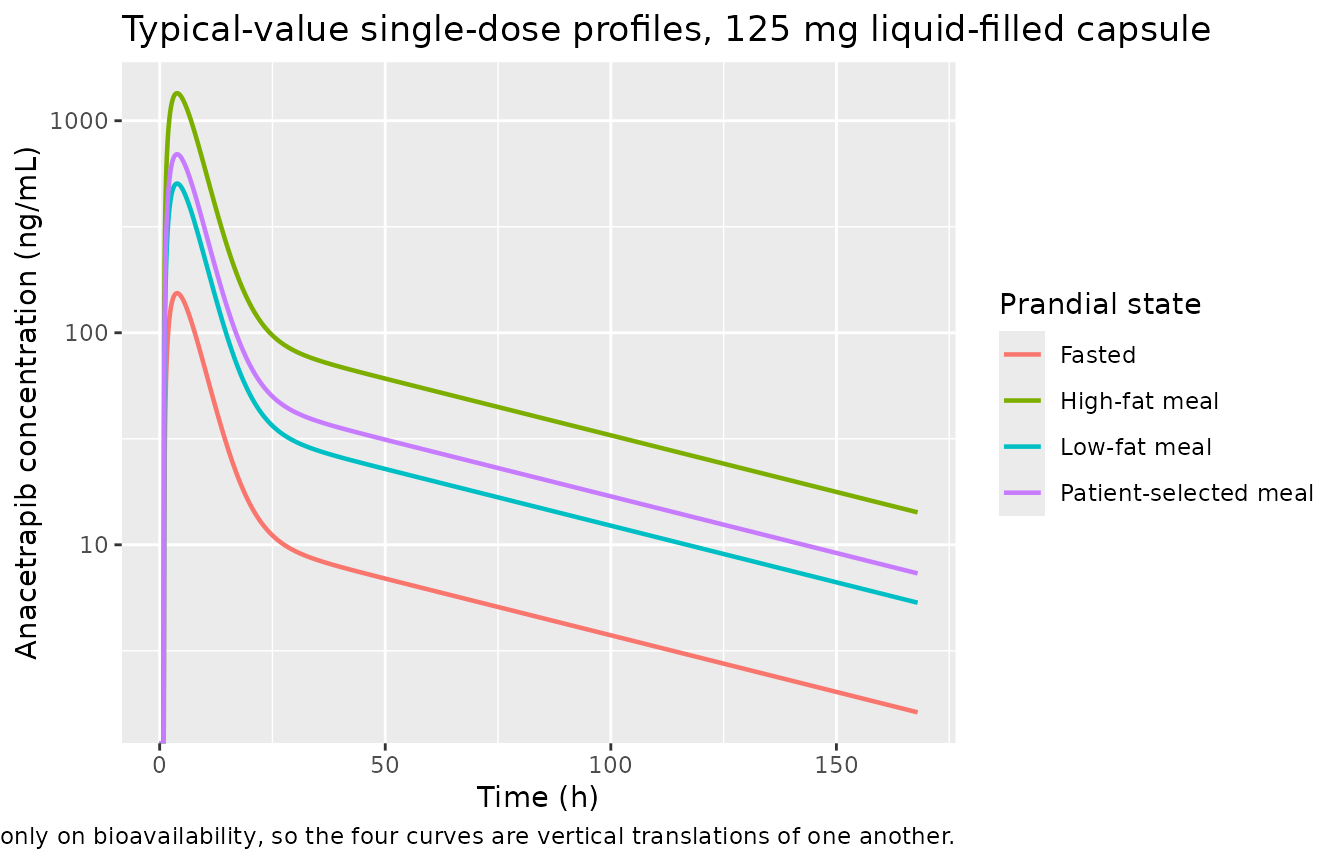

sim_nca <- food_sim |>
  dplyr::filter(!is.na(Cc)) |>
  dplyr::select(id, time, Cc, treatment)

# Guarantee a time-zero row per (id, treatment); pre-dose Cc = 0 is correct for
# extravascular dosing. Adding `time > 0` or `Cc > 0` to the filter above would
# drop it and trigger PKNCA's "AUC range starting before the first measurement".
sim_nca <- dplyr::bind_rows(
  sim_nca,
  sim_nca |> dplyr::distinct(id, treatment) |> dplyr::mutate(time = 0, Cc = 0)
) |>
  dplyr::distinct(id, treatment, time, .keep_all = TRUE) |>
  dplyr::arrange(id, treatment, time)

conc_obj <- PKNCA::PKNCAconc(sim_nca, Cc ~ time | treatment + id,
                             concu = "ng/mL", timeu = "h")

dose_df <- food_events |>
  dplyr::filter(evid == 1) |>
  dplyr::select(id, time, amt, treatment)
dose_obj <- PKNCA::PKNCAdose(dose_df, amt ~ time | treatment + id, doseu = "mg")

intervals <- data.frame(
  start      = 0,
  end        = Inf,
  cmax       = TRUE,
  tmax       = TRUE,
  aucinf.obs = TRUE,
  half.life  = TRUE
)

nca_res <- PKNCA::pk.nca(PKNCA::PKNCAdata(conc_obj, dose_obj,
                                          intervals = intervals))

nca_wide <- as.data.frame(nca_res$result) |>
  dplyr::select(treatment, PPTESTCD, PPORRES) |>
  tidyr::pivot_wider(names_from = PPTESTCD, values_from = PPORRES)

Check 1 – AUC against its closed form

For any linear model with complete absorption of F1 * dose, AUC(0-inf) = F1 * dose / CL. With dose in mg, CL in L/h and concentrations in ng/mL that is 1000 * F1 * dose / CL. This is the single cheapest falsifier of a mis-transcribed clearance or bioavailability term, and it is exact.

f1_by_state <- c("Fasted" = f1_of(125, lfc = 1),
                 "Low-fat meal" = f1_of(125, lf = 1, lfc = 1),
                 "Patient-selected meal" = f1_of(125, pb = 1, lfc = 1),
                 "High-fat meal" = f1_of(125, hf = 1, lfc = 1))
#> ℹ omega/sigma items treated as zero: 'etalcl', 'etalfdepot'
#> ℹ omega/sigma items treated as zero: 'etalcl', 'etalfdepot'
#> ℹ omega/sigma items treated as zero: 'etalcl', 'etalfdepot'
#> ℹ omega/sigma items treated as zero: 'etalcl', 'etalfdepot'

auc_chk <- nca_wide |>
  dplyr::mutate(
    closed_form = 1000 * f1_by_state[treatment] * 125 / exp(pk_ui$theta[["lcl"]]),
    pct_diff    = 100 * (aucinf.obs - closed_form) / closed_form
  )

auc_chk |>
  dplyr::select(treatment, aucinf.obs, closed_form, pct_diff) |>
  dplyr::rename(
    "Prandial state"                 = treatment,
    "AUC(0-inf), PKNCA (`ng*h/mL`)"  = aucinf.obs,
    "1000 * F1 * dose / CL"          = closed_form,
    "Difference (%)"                 = pct_diff
  ) |>
  knitr::kable(digits = c(0, 1, 1, 5),
               caption = "PKNCA AUC against its closed form. Both sides use the same drawn parameters, so the only difference is integrator and trapezoidal error; a tight bound is correct here.")

PKNCA AUC against its closed form. Both sides use the same drawn parameters, so the only difference is integrator and trapezoidal error; a tight bound is correct here.
Prandial state	AUC(0-inf), PKNCA (`ng*h/mL`)	1000 * F1 * dose / CL	Difference (%)
Fasted	2196.2	2196.2	0.00119
High-fat meal	19270.3	19270.1	0.00119
Low-fat meal	7222.5	7222.4	0.00119
Patient-selected meal	9930.9	9930.8	0.00119


stopifnot(all(abs(auc_chk$pct_diff) < 0.1))

Check 2 – terminal half-life against the eigenvalue

th   <- pk_ui$theta
kel  <- exp(th[["lcl"]]) / exp(th[["lvc"]])
k12  <- exp(th[["lq"]])  / exp(th[["lvc"]])
k21  <- exp(th[["lq"]])  / exp(th[["lvp"]])
sm   <- kel + k12 + k21
beta <- (sm - sqrt(sm^2 - 4 * kel * k21)) / 2
t_half_closed <- log(2) / beta

cat(sprintf("closed-form terminal half-life: %.1f h\n", t_half_closed))
#> closed-form terminal half-life: 56.3 h
cat(sprintf("PKNCA half-life (range over the four arms): %.1f to %.1f h\n",
            min(nca_wide$half.life), max(nca_wide$half.life)))
#> PKNCA half-life (range over the four arms): 56.1 to 56.1 h

stopifnot(abs(mean(nca_wide$half.life) - t_half_closed) < 1)

A 56 h terminal half-life with once-daily dosing is why the paper’s clinical trial simulations found the lipid effects insensitive to occasional dietary indiscretion: a single high-fat or fasted day is heavily damped by the time it reaches the trough.

Check 3 – the food effect on AUC, and where the model does not reproduce Cmax

Krishna 2011’s Discussion reports, for the LFC, that “a standard low-fat meal increased the exposure of anacetrapib by approximately 3.6-fold and increased the Cmax by approximately 6-fold relative to the fasted state. A high-fat meal increased the AUC of anacetrapib by approximately 9-fold and increased Cmax by approximately 18-fold.”

ref <- nca_wide |> dplyr::filter(treatment == "Fasted")

food_chk <- nca_wide |>
  dplyr::filter(treatment != "Fasted") |>
  dplyr::mutate(
    auc_fold        = aucinf.obs / ref$aucinf.obs,
    cmax_fold       = cmax / ref$cmax,
    auc_published   = c("Low-fat meal" = 3.6, "Patient-selected meal" = NA,
                        "High-fat meal" = 9)[treatment],
    cmax_published  = c("Low-fat meal" = 6, "Patient-selected meal" = NA,
                        "High-fat meal" = 18)[treatment]
  )

food_chk |>
  dplyr::select(treatment, auc_fold, auc_published, cmax_fold, cmax_published) |>
  dplyr::rename(
    "Prandial state"          = treatment,
    "AUC fold (model)"        = auc_fold,
    "AUC fold (Krishna 2011)" = auc_published,
    "Cmax fold (model)"       = cmax_fold,
    "Cmax fold (Krishna 2011)" = cmax_published
  ) |>
  knitr::kable(digits = 2,
               caption = "Fed/fasted exposure ratios for the 125 mg liquid-filled capsule, against the observed ratios quoted in the Discussion. The paper reports no patient-selected food-effect ratio.")

Fed/fasted exposure ratios for the 125 mg liquid-filled capsule, against the observed ratios quoted in the Discussion. The paper reports no patient-selected food-effect ratio.
Prandial state	AUC fold (model)	AUC fold (Krishna 2011)	Cmax fold (model)	Cmax fold (Krishna 2011)
High-fat meal	8.77	9.0	8.77	18
Low-fat meal	3.29	3.6	3.29	6
Patient-selected meal	4.52	NA	4.52	NA


# The AUC ratios are reproduced. The high-fat ratio is a genuine test of the
# theta_D term, because it combines the prandial multiplier with the shift in
# the half-maximal dose.
hf <- food_chk |> dplyr::filter(treatment == "High-fat meal")
lf <- food_chk |> dplyr::filter(treatment == "Low-fat meal")
stopifnot(abs(hf$auc_fold - 9)   < 1)
stopifnot(abs(lf$auc_fold - 3.6) < 0.6)

The Cmax column is a known limitation of the published model, not of this implementation. The final model applies the prandial covariate to bioavailability only – there is no food effect on ka or on ltlag in Table I – so every prandial state scales the whole profile by the same factor and the model’s Cmax ratio necessarily equals its AUC ratio. The observed 6-fold and 18-fold Cmax ratios come from separate biopharmaceutics work that the Discussion cites as unpublished data, and the model does not attempt to capture them. That is a defensible design choice for this paper, whose entire PD layer is driven by the trough: the Discussion notes that “of the three key pharmacokinetic parameters, the C24h parameter was relatively less influenced both in magnitude and variability, in the presence of food.”

Check 4 – dose non-proportionality and accumulation

dp_events <- dplyr::bind_rows(lapply(seq_along(c(50, 100, 150, 300)), function(i) {
  d <- c(50, 100, 150, 300)[i]
  sd_events(d, paste0(d, " mg"), lf = 1, id_offset = 10L * i)
}))
dp_sim <- rxode2::rxSolve(pk_typ, dp_events, keep = c("treatment"),
                          returnType = "data.frame", addDosing = FALSE)
#> ℹ omega/sigma items treated as zero: 'etalcl', 'etalfdepot'
#> Warning: multi-subject simulation without without 'omega'

dp_auc <- dp_sim |>
  dplyr::filter(!is.na(Cc)) |>
  dplyr::group_by(treatment) |>
  dplyr::summarise(
    dose = dplyr::first(DOSE),
    # trapezoidal AUC to the end of the 600 h window; the closed-form check
    # above already validated PKNCA against F1*dose/CL, so a light integral is
    # sufficient for a shape comparison.
    auc  = sum(diff(time) * (head(Cc, -1) + tail(Cc, -1)) / 2),
    .groups = "drop"
  ) |>
  dplyr::arrange(dose) |>
  dplyr::mutate(auc_per_mg = auc / dose)

dp_auc |>
  dplyr::select(treatment, auc, auc_per_mg) |>
  dplyr::rename(
    "Dose (HME tablet, low-fat)"            = treatment,
    "AUC(0-600 h) (`ng*h/mL`)"              = auc,
    "Dose-normalised AUC (`ng*h/mL` per mg)" = auc_per_mg
  ) |>
  knitr::kable(digits = 1,
               caption = "Single-dose exposure over 50-300 mg. Krishna 2011 Discussion: 'the AUC0-inf, Cmax, and C24h increased in a less than dose proportional manner in the 50 to 300 mg dose range.'")

Single-dose exposure over 50-300 mg. Krishna 2011 Discussion: ‘the AUC0-inf, Cmax, and C24h increased in a less than dose proportional manner in the 50 to 300 mg dose range.’
Dose (HME tablet, low-fat)	AUC(0-600 h) (`ng*h/mL`)	Dose-normalised AUC (`ng*h/mL` per mg)
50 mg	8268.9	165.4
100 mg	11203.1	112.0
150 mg	12705.9	84.7
300 mg	14674.4	48.9


# Deterministic and strongly monotone (the dose-normalised AUC falls roughly
# 3.4-fold across the range), so exact monotonicity is a legitimate assertion
# here -- there is no cohort and no random draw.
stopifnot(all(diff(dp_auc$auc_per_mg) < 0))
stopifnot(dp_auc$auc_per_mg[1] / dp_auc$auc_per_mg[nrow(dp_auc)] > 2)

tau <- 24
acc_grid <- sort(unique(c(seq(0, tau, by = 0.1), seq(tau * 89, tau * 90, by = 0.1))))
acc_ev <- rxode2::et(amt = 100, ii = tau, until = tau * 89, cmt = "depot")
acc_ev <- rxode2::et(acc_ev, acc_grid, cmt = "central")
acc_d  <- as.data.frame(acc_ev)
acc_d$id <- 1L
acc_d$DOSE <- 100
acc_d$FED_HIGHFAT <- 0
acc_d$FED_LOWFAT <- 1
acc_d$FED_PATIENTSELECTED <- 0
acc_d$FORM_ANACETRAPIB_LFC <- 0
acc_d$NDOSEUNITS <- 1

acc_sim <- rxode2::rxSolve(pk_typ, acc_d, returnType = "data.frame",
                           addDosing = FALSE) |>
  dplyr::filter(!is.na(Cc))
#> ℹ omega/sigma items treated as zero: 'etalcl', 'etalfdepot'

trap <- function(x, y) sum(diff(x) * (head(y, -1) + tail(y, -1)) / 2)
first_i <- acc_sim |> dplyr::filter(time <= tau)
ss_i    <- acc_sim |> dplyr::filter(time >= tau * 89)

acc_tab <- tibble::tibble(
  metric = c("Cmax", "AUC over the dosing interval"),
  ratio  = c(max(ss_i$Cc) / max(first_i$Cc),
             trap(ss_i$time, ss_i$Cc) / trap(first_i$time, first_i$Cc))
)

acc_tab |>
  dplyr::rename("Metric" = metric,
                "Steady state / first dose" = ratio) |>
  knitr::kable(digits = 2,
               caption = "Accumulation for 100 mg once daily as an HME tablet with a low-fat meal. Krishna 2011 Discussion: 'Multiple dose accumulation in the 50 to 300 mg dose range when administered with a low-fat meal as an HME tablet was approximately 1.2-1.9-fold.'")

Accumulation for 100 mg once daily as an HME tablet with a low-fat meal. Krishna 2011 Discussion: ‘Multiple dose accumulation in the 50 to 300 mg dose range when administered with a low-fat meal as an HME tablet was approximately 1.2-1.9-fold.’
Metric	Steady state / first dose
Cmax	1.24
AUC over the dosing interval	1.55


stopifnot(all(acc_tab$ratio > 1.2 & acc_tab$ratio < 1.9))

Coupling the PK layer to the PD layers

This is the step the paper describes as its population-simulation algorithm: compute the population-predicted trough concentration for a treatment condition, then evaluate the lipid response at that trough. The PK random effects are zeroed deliberately, because Table III’s PD variances were estimated against a population-predicted driver – propagating PK between-subject variability into CSS_ANACETRAPIB would double-count it.

ss_trough <- function(dose, hf = 0, lf = 0, pb = 0, lfc = 0, ncap = 1,
                      ndays = 90) {
  ev <- rxode2::et(amt = dose, ii = 24, until = 24 * (ndays - 1), cmt = "depot")
  ev <- rxode2::et(ev, seq(24 * (ndays - 1), 24 * ndays, by = 0.25),
                   cmt = "central")
  d  <- as.data.frame(ev)
  d$id <- 1L
  d$DOSE <- dose
  d$FED_HIGHFAT <- hf
  d$FED_LOWFAT <- lf
  d$FED_PATIENTSELECTED <- pb
  d$FORM_ANACETRAPIB_LFC <- lfc
  d$NDOSEUNITS <- ncap
  s <- rxode2::rxSolve(pk_typ, d, returnType = "data.frame",
                       addDosing = FALSE) |>
    dplyr::filter(!is.na(Cc))
  s$Cc[which.min(abs(s$time - 24 * ndays))]
}

# Confirm 90 days really is steady state for a drug with a 56 h terminal
# half-life before using the value as a gate input.
stopifnot(abs(ss_trough(100, pb = 1, ndays = 60) /
              ss_trough(100, pb = 1, ndays = 90) - 1) < 0.01)
#> ℹ omega/sigma items treated as zero: 'etalcl', 'etalfdepot'
#> ℹ omega/sigma items treated as zero: 'etalcl', 'etalfdepot'

hdl_typ <- rxode2::zeroRe(hdl_ui)
ldl_typ <- rxode2::zeroRe(ldl_ui)

pct_hdl <- function(css) {
  f <- function(x) {
    rxode2::rxSolve(hdl_typ, data.frame(id = 1L, time = 0,
                                        CSS_ANACETRAPIB = x),
                    returnType = "data.frame")$hdl
  }
  100 * (f(css) / f(0) - 1)
}

pct_ldl <- function(css, atorvastatin) {
  f <- function(x, a) {
    rxode2::rxSolve(ldl_typ,
                    data.frame(id = 1L, time = 0, CSS_ANACETRAPIB = x,
                               DIS_HYPERLIP = 1, CONMED_ATORVASTATIN = a),
                    returnType = "data.frame")$ldl
  }
  # Change from the untreated patient baseline, which is what the paper's
  # "% decrease in LDL-C" figures are relative to.
  100 * (f(css, atorvastatin) / f(0, 0) - 1)
}

anchors <- tibble::tribble(
  ~scenario,                                   ~dose, ~hf, ~pb, ~atv, ~endpoint,  ~published,
  "100 mg, patient-selected meal",               100,   0,   1,    0,  "HDL-C",     118,
  "100 mg, patient-selected meal",               100,   0,   1,    0,  "LDL-C",     -42,
  "100 mg, patient-selected meal + atorvastatin", 100,  0,   1,    1,  "LDL-C",     -67,
  "50 mg, fasted",                                50,   0,   0,    0,  "LDL-C",   -16.3,
  "50 mg, fasted + atorvastatin",                 50,   0,   0,    1,  "LDL-C",   -52.4,
  "50 mg, high-fat meal",                         50,   1,   0,    0,  "LDL-C",   -42.2,
  "50 mg, high-fat meal + atorvastatin",          50,   1,   0,    1,  "LDL-C",   -67.3,
  "Atorvastatin 20 mg alone",                      0,   0,   0,    1,  "LDL-C",   -44.2
)

anchors <- anchors |>
  dplyr::rowwise() |>
  dplyr::mutate(
    css = if (dose == 0) 0 else ss_trough(dose, hf = hf, pb = pb),
    simulated = if (endpoint == "HDL-C") pct_hdl(css) else pct_ldl(css, atv)
  ) |>
  dplyr::ungroup() |>
  dplyr::mutate(difference = simulated - published)
#> ℹ omega/sigma items treated as zero: 'etalcl', 'etalfdepot'
#> ℹ omega/sigma items treated as zero: 'etalcl', 'etalfdepot'
#> ℹ omega/sigma items treated as zero: 'etalcl', 'etalfdepot'
#> ℹ omega/sigma items treated as zero: 'etalcl', 'etalfdepot'
#> ℹ omega/sigma items treated as zero: 'etalcl', 'etalfdepot'
#> ℹ omega/sigma items treated as zero: 'etalcl', 'etalfdepot'
#> ℹ omega/sigma items treated as zero: 'etalcl', 'etalfdepot'
#> ℹ omega/sigma items treated as zero: 'etarbase', 'etaemax'
#> ℹ omega/sigma items treated as zero: 'etarbase', 'etaemax'
#> ℹ omega/sigma items treated as zero: 'etarbase'
#> ℹ omega/sigma items treated as zero: 'etarbase'
#> ℹ omega/sigma items treated as zero: 'etarbase'
#> ℹ omega/sigma items treated as zero: 'etarbase'
#> ℹ omega/sigma items treated as zero: 'etarbase'
#> ℹ omega/sigma items treated as zero: 'etarbase'
#> ℹ omega/sigma items treated as zero: 'etarbase'
#> ℹ omega/sigma items treated as zero: 'etarbase'
#> ℹ omega/sigma items treated as zero: 'etarbase'
#> ℹ omega/sigma items treated as zero: 'etarbase'
#> ℹ omega/sigma items treated as zero: 'etarbase'
#> ℹ omega/sigma items treated as zero: 'etarbase'
#> ℹ omega/sigma items treated as zero: 'etarbase'
#> ℹ omega/sigma items treated as zero: 'etarbase'

anchors |>
  dplyr::select(scenario, endpoint, css, simulated, published, difference) |>
  dplyr::rename(
    "Scenario"                        = scenario,
    "Endpoint"                        = endpoint,
    "Trough (ng/mL)"                  = css,
    "Change from baseline, % (model)" = simulated,
    "Change from baseline, % (Krishna 2011)" = published,
    "Difference (points)"             = difference
  ) |>
  knitr::kable(digits = 1,
               caption = "Reconstructed PK-to-PD chain against every lipid prediction Krishna 2011 publishes for a named treatment condition. Sources: Simulations of Efficacy Endpoints (the 50 mg rows and the atorvastatin-alone row) and the Discussion dose-selection paragraph (the 100 mg rows). No parameter was adjusted to obtain these.")

Reconstructed PK-to-PD chain against every lipid prediction Krishna 2011 publishes for a named treatment condition. Sources: Simulations of Efficacy Endpoints (the 50 mg rows and the atorvastatin-alone row) and the Discussion dose-selection paragraph (the 100 mg rows). No parameter was adjusted to obtain these.
Scenario	Endpoint	Trough (ng/mL)	Change from baseline, % (model)	Change from baseline, % (Krishna 2011)	Difference (points)
100 mg, patient-selected meal	HDL-C	276.4	118.2	118.0	0.2
100 mg, patient-selected meal	LDL-C	276.4	-43.1	-42.0	-1.1
100 mg, patient-selected meal + atorvastatin	LDL-C	276.4	-68.4	-67.0	-1.4
50 mg, fasted	LDL-C	61.8	-16.6	-16.3	-0.3
50 mg, fasted + atorvastatin	LDL-C	61.8	-53.5	-52.4	-1.1
50 mg, high-fat meal	LDL-C	276.6	-43.1	-42.2	-0.9
50 mg, high-fat meal + atorvastatin	LDL-C	276.6	-68.4	-67.3	-1.1
Atorvastatin 20 mg alone	LDL-C	0.0	-44.2	-44.2	0.0


# Typical-value throughout, so the only slack needed is for the paper's own
# rounding and for the fact that its published figures are means over 1,000
# parameter-uncertainty replicates while this is a point prediction. The
# achieved worst case is about 1.2 points.
stopifnot(max(abs(anchors$difference)) < 3)

Eight independent published predictions, spanning two endpoints, three doses, three prandial states and the atorvastatin interaction, reproduce to within about one percentage point. Two of them are worth calling out. The atorvastatin-alone row exercises theta_A on its own. The 100 mg patient-selected row is the paper’s actual phase III dose-selection decision: the threshold was a 40% LDL-C reduction, and the model puts it at 43%.

Pharmacologic independence

gamma = 0.99 is the paper’s headline pharmacological finding. The check below shows what that number means: setting gamma to exactly 1 makes the combined effect the exact product of the two monotherapy effects.

css100 <- ss_trough(100, pb = 1)
#> ℹ omega/sigma items treated as zero: 'etalcl', 'etalfdepot'

ldl_gamma1 <- rxode2::zeroRe(ldl_ui) |> rxode2::ini(e_conmed_atorvastatin_emax = 1)
#> ℹ change initial estimate of `e_conmed_atorvastatin_emax` to `1`
solve_ldl <- function(mod, css, atv) {
  rxode2::rxSolve(mod, data.frame(id = 1L, time = 0, CSS_ANACETRAPIB = css,
                                  DIS_HYPERLIP = 1, CONMED_ATORVASTATIN = atv),
                  returnType = "data.frame")$ldl
}

base   <- solve_ldl(ldl_gamma1, 0, 0)
#> ℹ omega/sigma items treated as zero: 'etarbase'
mono_a <- solve_ldl(ldl_gamma1, 0, 1)      / base   # atorvastatin alone
#> ℹ omega/sigma items treated as zero: 'etarbase'
mono_b <- solve_ldl(ldl_gamma1, css100, 0) / base   # anacetrapib alone
#> ℹ omega/sigma items treated as zero: 'etarbase'
combo  <- solve_ldl(ldl_gamma1, css100, 1) / base   # both
#> ℹ omega/sigma items treated as zero: 'etarbase'

cat(sprintf("gamma = 1: fraction of baseline, atorvastatin %.4f x anacetrapib %.4f = %.4f; combination solves to %.4f\n",
            mono_a, mono_b, mono_a * mono_b, combo))
#> gamma = 1: fraction of baseline, atorvastatin 0.5580 x anacetrapib 0.5693 = 0.3177; combination solves to 0.3177
stopifnot(abs(mono_a * mono_b - combo) < 1e-8)

# At the fitted gamma = 0.99 the departure from exact independence is tiny.
combo_fitted <- solve_ldl(ldl_typ, css100, 1) / solve_ldl(ldl_typ, 0, 0)
#> ℹ omega/sigma items treated as zero: 'etarbase'
#> ℹ omega/sigma items treated as zero: 'etarbase'
cat(sprintf("fitted gamma = 0.99: combination %.4f of baseline, vs %.4f under exact independence (%.2f points apart)\n",
            combo_fitted, mono_a * mono_b, 100 * (combo_fitted - mono_a * mono_b)))
#> fitted gamma = 0.99: combination 0.3158 of baseline, vs 0.3177 under exact independence (-0.19 points apart)
stopifnot(abs(combo_fitted - mono_a * mono_b) < 0.01)

Replicating Figure 4

Figure 4 of Krishna 2011 plots population-mean predicted HDL-C and LDL-C effects against dose, by prandial state, for monotherapy and for combination with atorvastatin 20 mg. It is a typical-value figure, so it is reproduced without between-subject variability.

doses <- c(10, 25, 50, 100, 150, 250, 300)
states <- tibble::tribble(
  ~state,                  ~hf, ~lf, ~pb,
  "Fasted",                  0,   0,   0,
  "Low-fat meal",            0,   1,   0,
  "Patient-selected meal",   0,   0,   1,
  "High-fat meal",           1,   0,   0
)

fig4 <- tidyr::crossing(states, dose = doses) |>
  dplyr::rowwise() |>
  dplyr::mutate(css = ss_trough(dose, hf = hf, lf = lf, pb = pb)) |>
  dplyr::mutate(
    `HDL-C, monotherapy`             = pct_hdl(css),
    `LDL-C, monotherapy`             = pct_ldl(css, 0),
    `LDL-C, + atorvastatin 20 mg`    = pct_ldl(css, 1)
  ) |>
  dplyr::ungroup() |>
  tidyr::pivot_longer(dplyr::starts_with(c("HDL-C", "LDL-C")),
                      names_to = "panel", values_to = "pct")
#> ℹ omega/sigma items treated as zero: 'etalcl', 'etalfdepot'
#> ℹ omega/sigma items treated as zero: 'etalcl', 'etalfdepot'
#> ℹ omega/sigma items treated as zero: 'etalcl', 'etalfdepot'
#> ℹ omega/sigma items treated as zero: 'etalcl', 'etalfdepot'
#> ℹ omega/sigma items treated as zero: 'etalcl', 'etalfdepot'
#> ℹ omega/sigma items treated as zero: 'etalcl', 'etalfdepot'
#> ℹ omega/sigma items treated as zero: 'etalcl', 'etalfdepot'
#> ℹ omega/sigma items treated as zero: 'etalcl', 'etalfdepot'
#> ℹ omega/sigma items treated as zero: 'etalcl', 'etalfdepot'
#> ℹ omega/sigma items treated as zero: 'etalcl', 'etalfdepot'
#> ℹ omega/sigma items treated as zero: 'etalcl', 'etalfdepot'
#> ℹ omega/sigma items treated as zero: 'etalcl', 'etalfdepot'
#> ℹ omega/sigma items treated as zero: 'etalcl', 'etalfdepot'
#> ℹ omega/sigma items treated as zero: 'etalcl', 'etalfdepot'
#> ℹ omega/sigma items treated as zero: 'etalcl', 'etalfdepot'
#> ℹ omega/sigma items treated as zero: 'etalcl', 'etalfdepot'
#> ℹ omega/sigma items treated as zero: 'etalcl', 'etalfdepot'
#> ℹ omega/sigma items treated as zero: 'etalcl', 'etalfdepot'
#> ℹ omega/sigma items treated as zero: 'etalcl', 'etalfdepot'
#> ℹ omega/sigma items treated as zero: 'etalcl', 'etalfdepot'
#> ℹ omega/sigma items treated as zero: 'etalcl', 'etalfdepot'
#> ℹ omega/sigma items treated as zero: 'etalcl', 'etalfdepot'
#> ℹ omega/sigma items treated as zero: 'etalcl', 'etalfdepot'
#> ℹ omega/sigma items treated as zero: 'etalcl', 'etalfdepot'
#> ℹ omega/sigma items treated as zero: 'etalcl', 'etalfdepot'
#> ℹ omega/sigma items treated as zero: 'etalcl', 'etalfdepot'
#> ℹ omega/sigma items treated as zero: 'etalcl', 'etalfdepot'
#> ℹ omega/sigma items treated as zero: 'etalcl', 'etalfdepot'
#> ℹ omega/sigma items treated as zero: 'etarbase', 'etaemax'
#> ℹ omega/sigma items treated as zero: 'etarbase', 'etaemax'
#> ℹ omega/sigma items treated as zero: 'etarbase', 'etaemax'
#> ℹ omega/sigma items treated as zero: 'etarbase', 'etaemax'
#> ℹ omega/sigma items treated as zero: 'etarbase', 'etaemax'
#> ℹ omega/sigma items treated as zero: 'etarbase', 'etaemax'
#> ℹ omega/sigma items treated as zero: 'etarbase', 'etaemax'
#> ℹ omega/sigma items treated as zero: 'etarbase', 'etaemax'
#> ℹ omega/sigma items treated as zero: 'etarbase', 'etaemax'
#> ℹ omega/sigma items treated as zero: 'etarbase', 'etaemax'
#> ℹ omega/sigma items treated as zero: 'etarbase', 'etaemax'
#> ℹ omega/sigma items treated as zero: 'etarbase', 'etaemax'
#> ℹ omega/sigma items treated as zero: 'etarbase', 'etaemax'
#> ℹ omega/sigma items treated as zero: 'etarbase', 'etaemax'
#> ℹ omega/sigma items treated as zero: 'etarbase', 'etaemax'
#> ℹ omega/sigma items treated as zero: 'etarbase', 'etaemax'
#> ℹ omega/sigma items treated as zero: 'etarbase', 'etaemax'
#> ℹ omega/sigma items treated as zero: 'etarbase', 'etaemax'
#> ℹ omega/sigma items treated as zero: 'etarbase', 'etaemax'
#> ℹ omega/sigma items treated as zero: 'etarbase', 'etaemax'
#> ℹ omega/sigma items treated as zero: 'etarbase', 'etaemax'
#> ℹ omega/sigma items treated as zero: 'etarbase', 'etaemax'
#> ℹ omega/sigma items treated as zero: 'etarbase', 'etaemax'
#> ℹ omega/sigma items treated as zero: 'etarbase', 'etaemax'
#> ℹ omega/sigma items treated as zero: 'etarbase', 'etaemax'
#> ℹ omega/sigma items treated as zero: 'etarbase', 'etaemax'
#> ℹ omega/sigma items treated as zero: 'etarbase', 'etaemax'
#> ℹ omega/sigma items treated as zero: 'etarbase', 'etaemax'
#> ℹ omega/sigma items treated as zero: 'etarbase', 'etaemax'
#> ℹ omega/sigma items treated as zero: 'etarbase', 'etaemax'
#> ℹ omega/sigma items treated as zero: 'etarbase', 'etaemax'
#> ℹ omega/sigma items treated as zero: 'etarbase', 'etaemax'
#> ℹ omega/sigma items treated as zero: 'etarbase', 'etaemax'
#> ℹ omega/sigma items treated as zero: 'etarbase', 'etaemax'
#> ℹ omega/sigma items treated as zero: 'etarbase', 'etaemax'
#> ℹ omega/sigma items treated as zero: 'etarbase', 'etaemax'
#> ℹ omega/sigma items treated as zero: 'etarbase', 'etaemax'
#> ℹ omega/sigma items treated as zero: 'etarbase', 'etaemax'
#> ℹ omega/sigma items treated as zero: 'etarbase', 'etaemax'
#> ℹ omega/sigma items treated as zero: 'etarbase', 'etaemax'
#> ℹ omega/sigma items treated as zero: 'etarbase', 'etaemax'
#> ℹ omega/sigma items treated as zero: 'etarbase', 'etaemax'
#> ℹ omega/sigma items treated as zero: 'etarbase', 'etaemax'
#> ℹ omega/sigma items treated as zero: 'etarbase', 'etaemax'
#> ℹ omega/sigma items treated as zero: 'etarbase', 'etaemax'
#> ℹ omega/sigma items treated as zero: 'etarbase', 'etaemax'
#> ℹ omega/sigma items treated as zero: 'etarbase', 'etaemax'
#> ℹ omega/sigma items treated as zero: 'etarbase', 'etaemax'
#> ℹ omega/sigma items treated as zero: 'etarbase', 'etaemax'
#> ℹ omega/sigma items treated as zero: 'etarbase', 'etaemax'
#> ℹ omega/sigma items treated as zero: 'etarbase', 'etaemax'
#> ℹ omega/sigma items treated as zero: 'etarbase', 'etaemax'
#> ℹ omega/sigma items treated as zero: 'etarbase', 'etaemax'
#> ℹ omega/sigma items treated as zero: 'etarbase', 'etaemax'
#> ℹ omega/sigma items treated as zero: 'etarbase', 'etaemax'
#> ℹ omega/sigma items treated as zero: 'etarbase', 'etaemax'
#> ℹ omega/sigma items treated as zero: 'etarbase'
#> ℹ omega/sigma items treated as zero: 'etarbase'
#> ℹ omega/sigma items treated as zero: 'etarbase'
#> ℹ omega/sigma items treated as zero: 'etarbase'
#> ℹ omega/sigma items treated as zero: 'etarbase'
#> ℹ omega/sigma items treated as zero: 'etarbase'
#> ℹ omega/sigma items treated as zero: 'etarbase'
#> ℹ omega/sigma items treated as zero: 'etarbase'
#> ℹ omega/sigma items treated as zero: 'etarbase'
#> ℹ omega/sigma items treated as zero: 'etarbase'
#> ℹ omega/sigma items treated as zero: 'etarbase'
#> ℹ omega/sigma items treated as zero: 'etarbase'
#> ℹ omega/sigma items treated as zero: 'etarbase'
#> ℹ omega/sigma items treated as zero: 'etarbase'
#> ℹ omega/sigma items treated as zero: 'etarbase'
#> ℹ omega/sigma items treated as zero: 'etarbase'
#> ℹ omega/sigma items treated as zero: 'etarbase'
#> ℹ omega/sigma items treated as zero: 'etarbase'
#> ℹ omega/sigma items treated as zero: 'etarbase'
#> ℹ omega/sigma items treated as zero: 'etarbase'
#> ℹ omega/sigma items treated as zero: 'etarbase'
#> ℹ omega/sigma items treated as zero: 'etarbase'
#> ℹ omega/sigma items treated as zero: 'etarbase'
#> ℹ omega/sigma items treated as zero: 'etarbase'
#> ℹ omega/sigma items treated as zero: 'etarbase'
#> ℹ omega/sigma items treated as zero: 'etarbase'
#> ℹ omega/sigma items treated as zero: 'etarbase'
#> ℹ omega/sigma items treated as zero: 'etarbase'
#> ℹ omega/sigma items treated as zero: 'etarbase'
#> ℹ omega/sigma items treated as zero: 'etarbase'
#> ℹ omega/sigma items treated as zero: 'etarbase'
#> ℹ omega/sigma items treated as zero: 'etarbase'
#> ℹ omega/sigma items treated as zero: 'etarbase'
#> ℹ omega/sigma items treated as zero: 'etarbase'
#> ℹ omega/sigma items treated as zero: 'etarbase'
#> ℹ omega/sigma items treated as zero: 'etarbase'
#> ℹ omega/sigma items treated as zero: 'etarbase'
#> ℹ omega/sigma items treated as zero: 'etarbase'
#> ℹ omega/sigma items treated as zero: 'etarbase'
#> ℹ omega/sigma items treated as zero: 'etarbase'
#> ℹ omega/sigma items treated as zero: 'etarbase'
#> ℹ omega/sigma items treated as zero: 'etarbase'
#> ℹ omega/sigma items treated as zero: 'etarbase'
#> ℹ omega/sigma items treated as zero: 'etarbase'
#> ℹ omega/sigma items treated as zero: 'etarbase'
#> ℹ omega/sigma items treated as zero: 'etarbase'
#> ℹ omega/sigma items treated as zero: 'etarbase'
#> ℹ omega/sigma items treated as zero: 'etarbase'
#> ℹ omega/sigma items treated as zero: 'etarbase'
#> ℹ omega/sigma items treated as zero: 'etarbase'
#> ℹ omega/sigma items treated as zero: 'etarbase'
#> ℹ omega/sigma items treated as zero: 'etarbase'
#> ℹ omega/sigma items treated as zero: 'etarbase'
#> ℹ omega/sigma items treated as zero: 'etarbase'
#> ℹ omega/sigma items treated as zero: 'etarbase'
#> ℹ omega/sigma items treated as zero: 'etarbase'
#> ℹ omega/sigma items treated as zero: 'etarbase'
#> ℹ omega/sigma items treated as zero: 'etarbase'
#> ℹ omega/sigma items treated as zero: 'etarbase'
#> ℹ omega/sigma items treated as zero: 'etarbase'
#> ℹ omega/sigma items treated as zero: 'etarbase'
#> ℹ omega/sigma items treated as zero: 'etarbase'
#> ℹ omega/sigma items treated as zero: 'etarbase'
#> ℹ omega/sigma items treated as zero: 'etarbase'
#> ℹ omega/sigma items treated as zero: 'etarbase'
#> ℹ omega/sigma items treated as zero: 'etarbase'
#> ℹ omega/sigma items treated as zero: 'etarbase'
#> ℹ omega/sigma items treated as zero: 'etarbase'
#> ℹ omega/sigma items treated as zero: 'etarbase'
#> ℹ omega/sigma items treated as zero: 'etarbase'
#> ℹ omega/sigma items treated as zero: 'etarbase'
#> ℹ omega/sigma items treated as zero: 'etarbase'
#> ℹ omega/sigma items treated as zero: 'etarbase'
#> ℹ omega/sigma items treated as zero: 'etarbase'
#> ℹ omega/sigma items treated as zero: 'etarbase'
#> ℹ omega/sigma items treated as zero: 'etarbase'
#> ℹ omega/sigma items treated as zero: 'etarbase'
#> ℹ omega/sigma items treated as zero: 'etarbase'
#> ℹ omega/sigma items treated as zero: 'etarbase'
#> ℹ omega/sigma items treated as zero: 'etarbase'
#> ℹ omega/sigma items treated as zero: 'etarbase'
#> ℹ omega/sigma items treated as zero: 'etarbase'
#> ℹ omega/sigma items treated as zero: 'etarbase'
#> ℹ omega/sigma items treated as zero: 'etarbase'
#> ℹ omega/sigma items treated as zero: 'etarbase'
#> ℹ omega/sigma items treated as zero: 'etarbase'
#> ℹ omega/sigma items treated as zero: 'etarbase'
#> ℹ omega/sigma items treated as zero: 'etarbase'
#> ℹ omega/sigma items treated as zero: 'etarbase'
#> ℹ omega/sigma items treated as zero: 'etarbase'
#> ℹ omega/sigma items treated as zero: 'etarbase'
#> ℹ omega/sigma items treated as zero: 'etarbase'
#> ℹ omega/sigma items treated as zero: 'etarbase'
#> ℹ omega/sigma items treated as zero: 'etarbase'
#> ℹ omega/sigma items treated as zero: 'etarbase'
#> ℹ omega/sigma items treated as zero: 'etarbase'
#> ℹ omega/sigma items treated as zero: 'etarbase'
#> ℹ omega/sigma items treated as zero: 'etarbase'
#> ℹ omega/sigma items treated as zero: 'etarbase'
#> ℹ omega/sigma items treated as zero: 'etarbase'
#> ℹ omega/sigma items treated as zero: 'etarbase'
#> ℹ omega/sigma items treated as zero: 'etarbase'
#> ℹ omega/sigma items treated as zero: 'etarbase'
#> ℹ omega/sigma items treated as zero: 'etarbase'
#> ℹ omega/sigma items treated as zero: 'etarbase'
#> ℹ omega/sigma items treated as zero: 'etarbase'
#> ℹ omega/sigma items treated as zero: 'etarbase'
#> ℹ omega/sigma items treated as zero: 'etarbase'
#> ℹ omega/sigma items treated as zero: 'etarbase'
#> ℹ omega/sigma items treated as zero: 'etarbase'
#> ℹ omega/sigma items treated as zero: 'etarbase'
#> ℹ omega/sigma items treated as zero: 'etarbase'

ggplot(fig4, aes(dose, pct, colour = state)) +
  geom_line(linewidth = 0.8) +
  geom_point(size = 1.2) +
  facet_wrap(~panel, scales = "free_y") +
  labs(x = "Anacetrapib dose (mg once daily, HME tablet)",
       y = "Population mean change from baseline (%)",
       colour = "Prandial state",
       title = "Population mean predicted HDL-C and LDL-C effects",
       caption = "Replicates Figure 4 of Krishna 2011 (panels a, b and c).")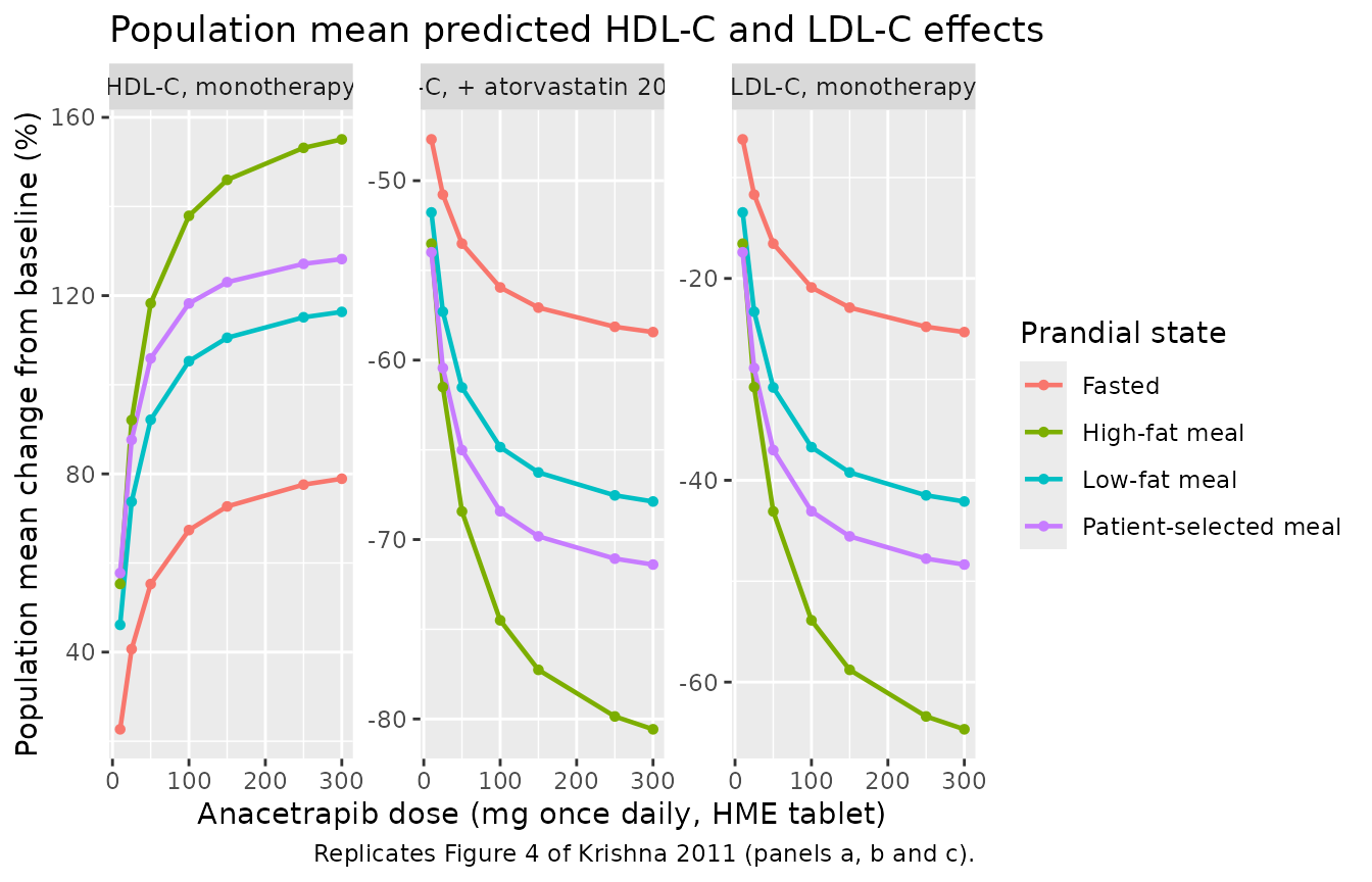

The figure reproduces the paper’s qualitative reading of it: the high-fat regimen gives the largest response and the fasted regimen the smallest, the low-fat and patient-selected regimens are close together, and both endpoints are near their plateau by 100 mg – which is the argument the paper used to stop at 100 mg for phase III.

at100 <- fig4 |> dplyr::filter(dose == 100)
at300 <- fig4 |> dplyr::filter(dose == 300)

# Typical-value throughout this section, so these are deterministic
# comparisons and not cohort statistics.
hdl100 <- at100 |> dplyr::filter(panel == "HDL-C, monotherapy")
stopifnot(hdl100$pct[hdl100$state == "High-fat meal"] >
            hdl100$pct[hdl100$state == "Fasted"])

# "Low-fat and patient-selected regimens reflect similar responses" -- the two
# differ by 13.0 points on HDL-C at 100 mg, against 70.5 points between fasted
# and high-fat, so a 25-point bound still separates "similar" from "different"
# by a factor of about three.
stopifnot(abs(hdl100$pct[hdl100$state == "Low-fat meal"] -
                hdl100$pct[hdl100$state == "Patient-selected meal"]) < 25)

# Plateau: "further increases in dose were not expected to lead to substantial
# additional efficacy". Tripling 100 mg to 300 mg adds at most 20% more effect
# on any panel in any prandial state (worst case observed: 20% on high-fat
# LDL-C monotherapy).
plateau <- dplyr::inner_join(
  at100 |> dplyr::select(state, panel, pct100 = pct),
  at300 |> dplyr::select(state, panel, pct300 = pct),
  by = c("state", "panel")
) |>
  dplyr::mutate(relative_gain = abs(pct300) / abs(pct100) - 1)
stopifnot(all(plateau$relative_gain < 0.30))

A cohort with between-subject variability

The checks above are all typical-value. This last section exercises the shipped IIV – the correlated cl / F1 block in the PK model and the additive baseline and Emax random effects in the PD models – on a cohort at the phase III regimen. It reproduces the shape of the visual-predictive checks in Figures 2 and 3 (lipid level against trough concentration) rather than a specific published number.

# rxSetSeed() fixes rxode2's stream per solver thread, not across thread
# counts, so the exact cohort below differs between machines. Every assertion
# in this section is written to hold for any cohort the model can produce.
rxode2::rxSetSeed(20261103)
n_per_arm <- 150L

# One rxSolve call per arm: rxSolve on an rxUi is quadratic in subject count
# when arms are stacked into a single call.
pk_cohort <- function(dose, label, hf = 0, lf = 0, pb = 0, id_offset = 0L) {
  ev <- rxode2::et(amt = dose, ii = 24, until = 24 * 89, cmt = "depot")
  ev <- rxode2::et(ev, seq(24 * 89, 24 * 90, by = 1), cmt = "central")
  d  <- as.data.frame(ev)
  d$DOSE <- dose
  d$FED_HIGHFAT <- hf
  d$FED_LOWFAT <- lf
  d$FED_PATIENTSELECTED <- pb
  d$FORM_ANACETRAPIB_LFC <- 0
  d$NDOSEUNITS <- 1
  d$arm <- label
  # With `nSub`, rxode2 keys subjects on `sim.id` rather than `id` (the input
  # event table carries no id column of its own). `Cc` is the individual
  # prediction; the residual-error draw is the separate `sim` column, and the
  # PD driver must be the prediction, not a noisy observation.
  s <- rxode2::rxSolve(pk_ui, d, nSub = n_per_arm, keep = c("arm"),
                       returnType = "data.frame") |>
    dplyr::filter(!is.na(Cc))
  s |>
    dplyr::group_by(sim.id) |>
    dplyr::summarise(css = Cc[which.max(time)], .groups = "drop") |>
    dplyr::transmute(id = sim.id + id_offset, css = css, arm = label)
}

cohort_css <- dplyr::bind_rows(
  pk_cohort(100, "100 mg, patient-selected", pb = 1, id_offset = 0L),
  pk_cohort(100, "100 mg, fasted",                   id_offset = 1000L),
  pk_cohort(300, "300 mg, patient-selected", pb = 1, id_offset = 2000L)
)
stopifnot(!anyDuplicated(cohort_css$id), all(cohort_css$css > 0))

cohort_pd <- cohort_css |>
  dplyr::mutate(DIS_HYPERLIP = 1, CONMED_ATORVASTATIN = 0, time = 0,
                CSS_ANACETRAPIB = css)

hdl_sim <- rxode2::rxSolve(hdl_ui, cohort_pd, keep = c("arm", "css"),
                           returnType = "data.frame")
ldl_sim <- rxode2::rxSolve(ldl_ui, cohort_pd, keep = c("arm", "css"),
                           returnType = "data.frame")

cohort_long <- dplyr::bind_rows(
  hdl_sim |> dplyr::transmute(arm, css, endpoint = "HDL-C (mg/dL)", value = hdl),
  ldl_sim |> dplyr::transmute(arm, css, endpoint = "LDL-C (mg/dL)", value = ldl)
)

ggplot(cohort_long, aes(css, value, colour = arm)) +
  geom_point(alpha = 0.35, size = 1) +
  facet_wrap(~endpoint, scales = "free_y") +
  labs(x = "Population-predicted anacetrapib trough (ng/mL)",
       y = "Steady-state lipid level (mg/dL)",
       colour = "Arm",
       title = paste0("Simulated cohort, ", n_per_arm, " subjects per arm"),
       caption = "Reproduces the shape of the visual-predictive checks in Figures 2 and 3 of Krishna 2011: lipid level against trough concentration, pooling arms.")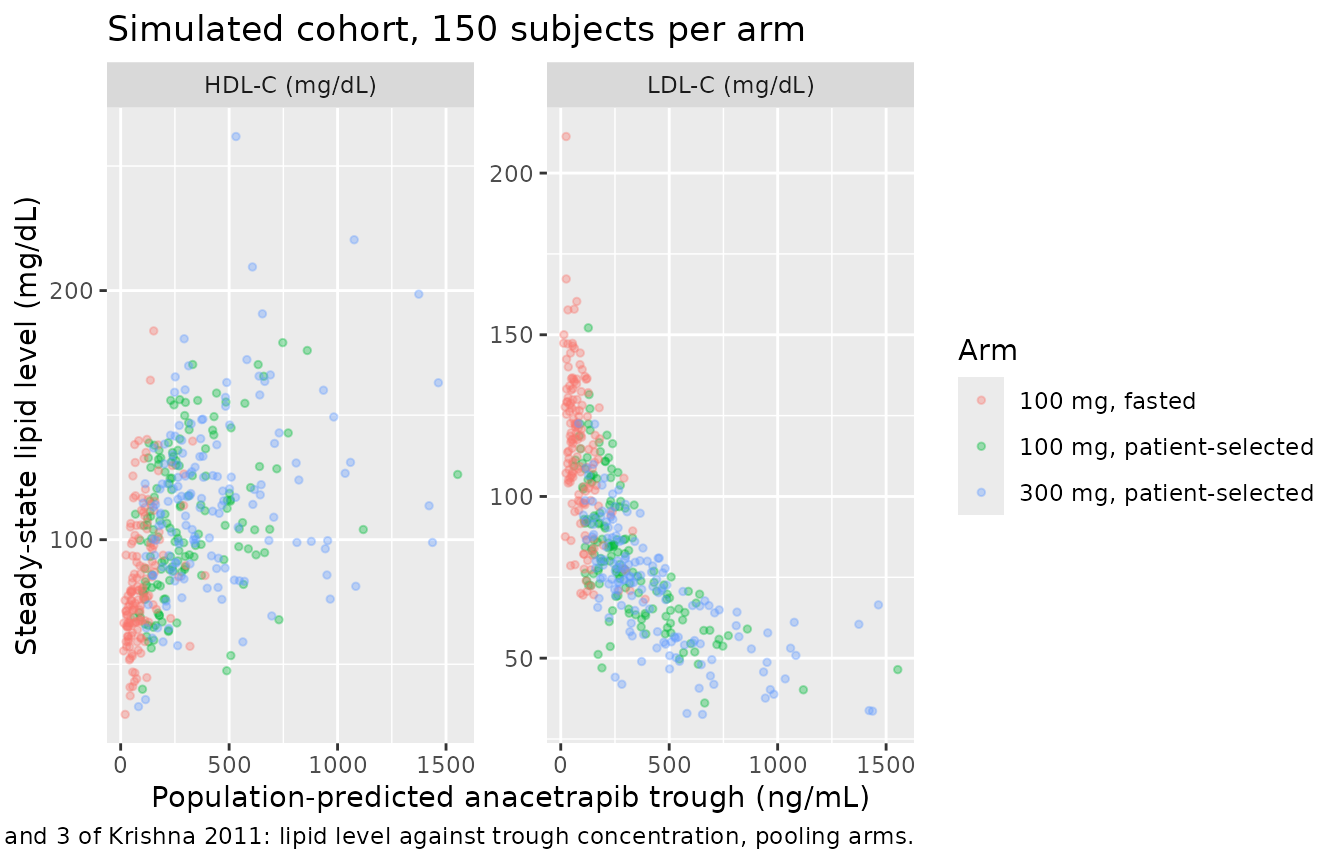

arm_summary <- cohort_long |>
  dplyr::group_by(arm, endpoint) |>
  dplyr::summarise(median = median(value),
                   q10 = quantile(value, 0.1),
                   q90 = quantile(value, 0.9),
                   .groups = "drop")

arm_summary |>
  dplyr::rename("Arm" = arm, "Endpoint" = endpoint, "Median" = median,
                "10th percentile" = q10, "90th percentile" = q90) |>
  knitr::kable(digits = 1,
               caption = "Cohort medians and 10th-90th percentile ranges. Compare against the typical-value predictions above; the medians sit close to them, while the spread reflects the shipped baseline and Emax variability.")

Cohort medians and 10th-90th percentile ranges. Compare against the typical-value predictions above; the medians sit close to them, while the spread reflects the shipped baseline and Emax variability.
Arm	Endpoint	Median	10th percentile	90th percentile
100 mg, fasted	HDL-C (mg/dL)	78.2	55.6	117.9
100 mg, fasted	LDL-C (mg/dL)	114.3	80.1	140.1
100 mg, patient-selected	HDL-C (mg/dL)	104.5	67.8	147.2
100 mg, patient-selected	LDL-C (mg/dL)	80.4	57.4	111.0
300 mg, patient-selected	HDL-C (mg/dL)	115.0	76.6	160.0
300 mg, patient-selected	LDL-C (mg/dL)	73.2	47.9	95.3


# Cohort-derived, so assert on the CENTRE against the typical-value
# prediction and never on the extremes. The typical value is obtained by
# solving the same model with the random effects zeroed, rather than by
# re-typing the equation, so the check cross-validates the two paths.
typical_100pb_hdl <- rxode2::rxSolve(
  hdl_typ,
  data.frame(id = 1L, time = 0, CSS_ANACETRAPIB = css100),
  returnType = "data.frame"
)$hdl
#> ℹ omega/sigma items treated as zero: 'etarbase', 'etaemax'
med_hdl <- arm_summary$median[arm_summary$arm == "100 mg, patient-selected" &
                                arm_summary$endpoint == "HDL-C (mg/dL)"]
cat(sprintf("100 mg patient-selected HDL-C: typical value %.1f mg/dL, cohort median %.1f mg/dL\n",
            typical_100pb_hdl, med_hdl))
#> 100 mg patient-selected HDL-C: typical value 110.9 mg/dL, cohort median 104.5 mg/dL
# The baseline random effect is additive and symmetric, so the median tracks
# the typical value closely; 8 mg/dL is well outside the run-to-run spread
# (under a mg/dL on the median) while still far tighter than the 23% baseline
# CV the model carries.
stopifnot(abs(med_hdl - typical_100pb_hdl) < 8)

# LDL-C is bounded below by the Emax asymptote, rbase_i * (1 + emax), which is
# 28 mg/dL at the typical patient baseline. Positivity is structural, not a
# cohort statistic.
stopifnot(all(ldl_sim$ldl > 0))
# Higher trough -> lower LDL-C. Both arms differ by roughly a factor of three
# in trough concentration, so the median ordering is not a close race.
stopifnot(median(ldl_sim$ldl[ldl_sim$arm == "300 mg, patient-selected"]) <
            median(ldl_sim$ldl[ldl_sim$arm == "100 mg, fasted"]))

Assumptions and deviations

Random-effect and residual-error scales differ between the PK and PD tables, and both readings are forced by internal evidence. Table I (NONMEM) reports omega_CL = 0.098, omega_F1 = 0.21 and Cov = 0.04. Those must be variances: reading the diagonals as standard deviations would give a correlation of 0.04 / sqrt(0.0096 * 0.0441) = 1.94, which is impossible. The sigma rows of the same table are read on the same variance scale by parallel construction, so the model ships propSd = sqrt(0.184) = 0.429 and addSd = sqrt(32.4) = 5.69 ng/mL. Tables II and III (S-PLUS NLME) go the other way and are read as standard deviations: 11.7 mg/dL on a 50.8 mg/dL HDL-C baseline is a 23% coefficient of variation, whereas a variance reading would give 3.4 mg/dL (6.7% CV), far too small for population HDL-C; the same argument applies to the 25 mg/dL LDL-C figure. Neither table states its convention. A user who prefers the alternative reading can change it in one line (ini(propSd = 0.184), etc.); nothing else in the model depends on it, and none of the validation checks in this vignette are affected, because all of the tight ones are typical-value.

The dosage-unit terms are gated on the formulation, which the equations do not print. Discussed under “Two readings that had to be recovered” above; the gating is stated in the Methods (“for LFC only”) and is the only reading that reproduces the paper’s four printed tablet bioavailability values.

Eq. 9’s interaction term was recovered as gamma * theta_A. Also discussed above. The literal rendering of the PDF is arithmetically falsified by the paper’s own worked example, and only the recovered reading gives gamma = 1 the meaning the paper assigns it.

Bioavailability above 1. F1 reaches 2.07 for a high-fat 100 mg tablet. The absolute scale of F1 is not identified separately from cl; the paper itself calls these “relative bioavailability”, and lfdepot is fixed at 1 as an anchor.

No food effect on absorption rate. The model reproduces the published fed/fasted AUC ratios but not the published Cmax ratios, because Table I contains no prandial effect on ka or ltlag. This is a property of the published model. See Check 3.

DOSE is supplied as a data column rather than read from the dose record. Eq. 6 needs the nominal dose. rxode2::podo() would also supply it, but a bare podo() call can silently return 0 through rxUi, which here would replace F1 = 0.35 with F1 = 1. Since Krishna 2011 describes dose_i as a per-subject covariate, the explicit column is both safer and closer to the source.

The fasted indicator is derived, not supplied. Following the register’s FED_* convention and the Hu_2026_utreloxastat precedent, the fasted state is the complement of the three fed indicators rather than a fourth column.

The 90-day run-in used to reach steady state is this vignette’s choice. The paper does not state a simulation duration. With a 56 h terminal half-life, 90 days is about 38 half-lives, and the vignette asserts that the day-60 and day-90 troughs agree to within 1%.

Cohort covariate distributions. The IIV section uses DIS_HYPERLIP = 1 for every subject (a dyslipidemic-patient cohort) and no atorvastatin. The paper’s own analysis set was 87% patients. No demographic covariate is in any of the three models, so no demographic distribution needed to be assumed.

Errata and source gaps

No erratum or corrigendum to Krishna 2011 was located.

The Electronic Supplementary Material is not on disk. It holds Table IA and Table IB (per-study designs: doses, formulations, sampling schedules and per-study subject counts) and five supplementary diagnostic figures. Every parameter of all three models is in the main-text tables, so the gap costs demographic and per-study detail only, and it is the reason population$age_range, weight_range, sex_female_pct and race_ethnicity are absent from all three model files rather than populated. An attempt to retrieve it on 2026-09-03 failed: the EuropePMC supplementaryFiles endpoint returned HTTP 504 for both this PMCID and a control PMCID (so an outage, not a missing deposit), and the Springer static-content route returned HTTP 403.

The trimmed markdown of this paper is unusable for the equations. All nine display equations render as formula-not-decoded, and the PDF’s symbol font encodes multiplication signs, minus signs and Greek letters as C0 control bytes that pdftotext silently drops. The equations in this vignette were recovered with pdftotext -layout plus cat -A and then confirmed numerically against the fifteen published predictions checked above, rather than trusted as printed.

Upstream dependency. Krishna 2011’s higher-atorvastatin-dose extrapolations lean on the Mandema 2005 statin dose-response meta-analysis (reference 6), which is not part of any model shipped here. Only the atorvastatin 20 mg indicator was fitted in this paper, and CONMED_ATORVASTATIN should not be reinterpreted as a generic statin flag.

Reported but not modelled. The paper’s clinical trial simulations of dietary non-compliance (75% low-fat / 25% fasting, Fig. 5) are a study-design exercise on top of these three models rather than additional model structure, and are not reproduced here.