Durvalumab (Abegesah 2025)
Source:vignettes/articles/Abegesah_2025_durvalumab.Rmd
Abegesah_2025_durvalumab.RmdModel and source
- Citation: Abegesah A, Oh D-Y, Lim K, Fan C, Chen C, Kim C, Wang J, Xynos I, Zotkiewicz M, Ren S, Phipps A, Gibbs M, Zhou D. Population pharmacokinetics and exposure-response analysis of durvalumab in combination with gemcitabine and cisplatin in patients with advanced biliary tract cancer. Cancer Chemother Pharmacol. 2025;95:23. doi:10.1007/s00280-024-04743-8
- Description: Two-compartment population PK model for durvalumab (anti-PD-L1 IgG1 kappa) with sigmoidal time-varying clearance in adults with advanced solid tumours, updating the POSEIDON model with TOPAZ-1 biliary tract cancer patients treated with durvalumab plus gemcitabine/cisplatin (Abegesah 2025)
- Article: https://doi.org/10.1007/s00280-024-04743-8
- Supplement (Table S1, Figs. S1-S3): https://doi.org/10.1007/s00280-024-04743-8,
Supplementary Appendix
280_2024_4743_MOESM1_ESM.docx
Abegesah 2025 updates the durvalumab POSEIDON population PK model by adding the phase III TOPAZ-1 cohort (advanced biliary tract cancer, durvalumab 1500 mg Q3W with gemcitabine/cisplatin) to the five previously analysed studies. The structure is two-compartment with linear clearance and a sigmoidal time-dependent clearance component; the analysis added tumor type on clearance as its only new covariate.
The paper’s exposure-response analyses are not
represented by a packaged model, and deliberately so: the
overall-survival analysis is a Cox proportional hazards model whose
baseline hazard h0(t) is never reported (Table 3 gives only
the three covariate coefficients), and the safety analyses found no
exposure-response relationship and therefore report no fitted logistic
coefficients at all. Neither is simulatable from what is on the page.
See Assumptions and deviations below.
Population
The pooled analysis dataset comprises 3141 patients from six studies (Table 1): Study 1108 (phase 1/2, advanced solid tumours, n = 1012), ATLANTIC (phase 2, NSCLC, n = 443), PACIFIC (phase 3, unresectable stage III NSCLC, n = 473), CASPIAN (phase 3, extensive-disease SCLC, n = 260), POSEIDON (phase 3, metastatic NSCLC, n = 326) and TOPAZ-1 (phase 3, advanced BTC, n = 314).
Baseline characteristics (Table 2) are a median age of 63 years (19-96), median weight 69.0 kg (31.0-175), 36.6% female, and White 67.2% / Asian 26.2% / Black 2.5% / Other 4.2%. Median baseline albumin was 39.0 g/L, creatinine clearance 85.9 mL/min and LDH 242 U/L. ECOG performance status was 0 in 37.9% and 1 in 61.8%. Treatment was durvalumab monotherapy in 60.3%, durvalumab + chemotherapy in 28.2% (which includes all 314 TOPAZ-1 patients) and durvalumab + tremelimumab + chemotherapy in 10.3%. Treatment-emergent ADA positivity was 3.53%, and exposure was comparable between ADA-positive and ADA-negative patients.
The TOPAZ-1 subgroup that drives the validation below is younger-weighted and more Asian than the pool: median age 64 years (20-84), median weight 63.0 kg (36.5-127), 50.6% female, Asian 53.1% / White 40.9%, median albumin 39.0 g/L, creatinine clearance 87.9 mL/min and LDH 217 U/L.
A reference-value trap worth flagging. The covariate normalizers printed inside the model equations (weight 69.4 kg, LDH 247 U/L, creatinine clearance 85.66 mL/min) are the Previous 5 studies medians of Table 2, i.e. the reference patient inherited from the POSEIDON model – not the pooled 6-study medians of this analysis (69.0 kg, 242 U/L, 85.9 mL/min). The two columns sit side by side in Table 2 and are easy to swap.
The same information is available programmatically via the model’s
population metadata
(readModelDb("Abegesah_2025_durvalumab")()$population).
Source trace
Every ini() entry in
inst/modeldb/specificDrugs/Abegesah_2025_durvalumab.R
carries an in-file comment naming its source location. They are
collected here for review.
| Equation / parameter | Value | Source location |
|---|---|---|
lcl (CL) |
0.298 L/day | Table 4, “CL” |
lvc (V1) |
3.42 L | Table 4, “V1” |
lq (Q) |
0.452 L/day | Table 4, “Q” |
lvp (V2) |
1.99 L | Table 4, “V2” |
cl_time_max |
-0.498 | Table 4, “Tmax change CL” |
cl_t50 |
61.3 days | Table 4, “TC50 change CL” |
cl_time_hill |
1.00 (fixed) | Table 4, “LAM” (no RSE, no CI) |
e_alb_cl |
-0.589 | Table 4, “Albumin on CL”; page 3 CL_cont.cov
|
e_crcl_cl |
0.136 | Table 4, “CrCL on CL”; page 3 CL_cont.cov
|
e_ldh_cl |
0.0515 | Table 4, “LDH on CL”; page 3 CL_cont.cov
|
e_wt_cl |
0.338 | Table 4, “Body weight on CL”; page 3 CL_cont.cov
|
e_ecog_cl |
-0.0501 | Table 4, “ECOG status on CL”; page 3 CL_cat.cov
|
e_sexf_cl |
-0.161 | Table 4, “Sex on CL”; page 3 CL_cat.cov
|
e_chemo_cl |
-0.163 | Table 4, “COMB1 on CL”; page 3 CL_cat.cov; Fig. 1
“Combo Durva + Chemo” |
e_treme_cl |
-0.0929 | Table 4, “COMB2 on CL”; page 3 CL_cat.cov; Fig. 1
“Combo Durva + Treme + Chemo” |
e_tumtp_other_cl |
-0.0101 | Page 3 CL_cat.cov (Table 4 “Tumor type 1 on CL” prints
+0.0101; see Errata) |
e_tumtp_bladder_cl |
0.0698 | Table 4, “Tumor type 2 on CL”; Fig. 1 “TUM TYP Bladder” (+7%) |
e_tumtp_btc_cl |
0.166 | Table 4, “Tumor type 3 on CL”; Fig. 1 “TUM TYP BTC” (+16.6%) |
e_wt_vc |
0.515 | Table 4, “Body weight on V1”; page 3 Vc equation |
e_sexf_vc |
-0.140 | Table 4, “Sex on V1”; page 3 Vc equation |
etalcl, etalvc, covariance |
0.0795, 0.0593, 0.0390 | Table 4, “ETA CL”, “ETA V1”, “Cov CL-V1” |
etacl_time_max |
0.0623 | Table 4, “ETA Tmax” |
propSd |
0.255 | Table 4, “Proportional component” |
addSd |
4.75 ug/mL | Table 4, “Additive component” |
| Covariate reference values 39 g/L, 85.66 mL/min, 247 U/L, 69.4 kg | n/a | Printed inside the CL_cont.cov and Vc
equations, page 3 |
CL_cat.cov, CL_cont.cov,
CL_T,i, Vc,i equations |
n/a | Page 3, unnumbered equation block following “Model equations for CL and V1 are shown below” |
| Two-compartment ODE structure | n/a | Results, “The final durvalumab PopPK model was a 2-compartment model with linear CL and an additional time-dependent CL component” |
Deterministic checks
These checks use rxode2::zeroRe(), so both sides of each
comparison use the same (typical) parameter values and the difference is
pure arithmetic on the published covariate model. Tight bounds are
therefore appropriate here – unlike the cohort-based checks further
down.
mod <- readModelDb("Abegesah_2025_durvalumab")
mod_typical <- rxode2::zeroRe(mod)
#> ℹ parameter labels from comments will be replaced by 'label()'

# Reference patient: every covariate at the model's own reference value, male,
# ECOG 0, durvalumab monotherapy, reference tumor type.
ref_cov <- list(
  WT = 69.4, ALB = 39, CRCL = 85.66, LDH = 247,
  SEXF = 0, ECOG_GE1 = 0,
  CONMED_CHEMO = 0, CONMED_TREMELIMUMAB = 0,
  TUMTP_OTHER = 0, TUMTP_BLADDER = 0, TUMTP_BTC = 0
)

# Solve a single 1500 mg 1 h infusion and return the requested columns.
solve_one <- function(cov, times = c(0, 21), amt = 1500) {
  ev <- rxode2::et(amt = amt, dur = 1 / 24, cmt = "central") |>
    rxode2::et(times, cmt = "central")
  d <- as.data.frame(ev)
  for (nm in names(cov)) d[[nm]] <- cov[[nm]]
  rxode2::rxSolve(mod_typical, d, returnType = "data.frame")
}

cl0 <- function(cov) solve_one(cov)$cl[1]
Time-dependent clearance asymptote (Abstract)
The Abstract states that “the clearance could decrease up to 39% over
the time course of treatment”. In the packaged model that claim is
1 - exp(cl_time_max).
asymptote_pct <- 100 * (1 - exp(-0.498))
asymptote_pct
#> [1] 39.22551

# Deterministic arithmetic on a published constant; no cohort noise involved.
stopifnot(abs(asymptote_pct - 39) < 0.5)
Half of that decrease is reached at cl_t50 = 61.3 days.
The trajectory of the typical TOPAZ-1 patient’s clearance over six Q3W
cycles:
topaz_typical <- list(
  WT = 63.0, ALB = 39.0, CRCL = 87.9, LDH = 217,
  SEXF = 0, ECOG_GE1 = 0,
  CONMED_CHEMO = 1, CONMED_TREMELIMUMAB = 0,
  TUMTP_OTHER = 0, TUMTP_BLADDER = 0, TUMTP_BTC = 1
)
cl_traj <- solve_one(topaz_typical, times = seq(0, 126, by = 1))
#> ℹ omega/sigma items treated as zero: 'etalcl', 'etalvc', 'etacl_time_max'

ggplot(cl_traj, aes(time, cl / cl[1])) +
  geom_line(linewidth = 0.8) +
  geom_hline(yintercept = exp(-0.498), linetype = "dashed", colour = "grey40") +
  geom_vline(xintercept = 61.3, linetype = "dotted", colour = "grey40") +
  labs(
    x = "Time (days)", y = "CL(t) / CL(0)",
    title = "Time-dependent clearance",
    caption = "Dashed: asymptote exp(-0.498) = 0.608. Dotted: TC50 = 61.3 days."
  )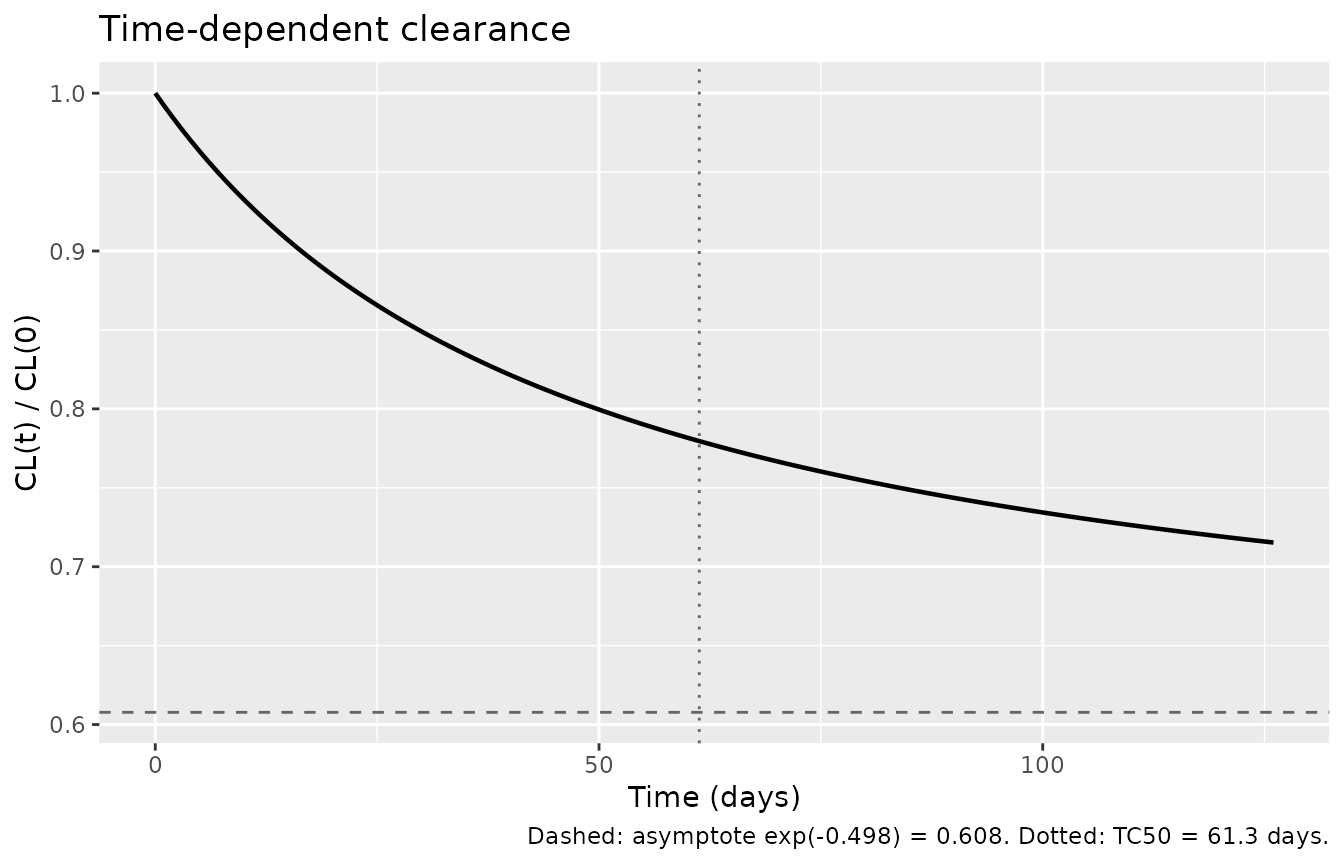
Time-dependent clearance of the typical TOPAZ-1 patient over 18 weeks, with the asymptotic 39.2% reduction shown as a dashed line.
Covariate impact on clearance (Fig. 1 and Results text)
The Results text quantifies three covariate effects explicitly: low baseline albumin (5th percentile) gives 19.1% higher CL, female sex gives 16.1% lower CL, and high body weight (95th percentile) gives 14.1% higher CL. Fig. 1 adds the remaining tornado bars. The percentiles Fig. 1 labels are albumin 29 g/L (5th) and 46 g/L (95th), creatinine clearance 49.6 and 152 mL/min, LDH 140 and 821 U/L, and body weight 47.6 and 102 kg.
bump <- function(field, value) {
  cov <- ref_cov
  cov[[field]] <- value
  100 * (cl0(cov) / cl0(ref_cov) - 1)
}

tornado <- tibble::tribble(
  ~term,                            ~published, ~simulated,
  "5th percentile BW (47.6 kg)",         -11.8, bump("WT", 47.6),
  "95th percentile BW (102 kg)",          14.1, bump("WT", 102),
  "5th percentile CRCL (49.6 mL/min)",    -7.2, bump("CRCL", 49.6),
  "95th percentile CRCL (152 mL/min)",     8.1, bump("CRCL", 152),
  "5th percentile Albumin (29 g/L)",      19.1, bump("ALB", 29),
  "95th percentile Albumin (46 g/L)",     -9.3, bump("ALB", 46),
  "5th percentile LDH (140 U/L)",         -2.8, bump("LDH", 140),
  "95th percentile LDH (821 U/L)",         6.5, bump("LDH", 821),
  "Female",                              -16.1, bump("SEXF", 1),
  "Combo Durva + Treme + Chemo",          -9.3, bump("CONMED_TREMELIMUMAB", 1),
  "Combo Durva + Chemo",                 -16.3, bump("CONMED_CHEMO", 1),
  "TUM TYP Bladder",                       7.0, bump("TUMTP_BLADDER", 1),
  "TUM TYP BTC",                          16.6, bump("TUMTP_BTC", 1)
) |>
  mutate(difference = simulated - published)
#> ℹ omega/sigma items treated as zero: 'etalcl', 'etalvc', 'etacl_time_max'
#> ℹ omega/sigma items treated as zero: 'etalcl', 'etalvc', 'etacl_time_max'
#> ℹ omega/sigma items treated as zero: 'etalcl', 'etalvc', 'etacl_time_max'
#> ℹ omega/sigma items treated as zero: 'etalcl', 'etalvc', 'etacl_time_max'
#> ℹ omega/sigma items treated as zero: 'etalcl', 'etalvc', 'etacl_time_max'
#> ℹ omega/sigma items treated as zero: 'etalcl', 'etalvc', 'etacl_time_max'
#> ℹ omega/sigma items treated as zero: 'etalcl', 'etalvc', 'etacl_time_max'
#> ℹ omega/sigma items treated as zero: 'etalcl', 'etalvc', 'etacl_time_max'
#> ℹ omega/sigma items treated as zero: 'etalcl', 'etalvc', 'etacl_time_max'
#> ℹ omega/sigma items treated as zero: 'etalcl', 'etalvc', 'etacl_time_max'
#> ℹ omega/sigma items treated as zero: 'etalcl', 'etalvc', 'etacl_time_max'
#> ℹ omega/sigma items treated as zero: 'etalcl', 'etalvc', 'etacl_time_max'
#> ℹ omega/sigma items treated as zero: 'etalcl', 'etalvc', 'etacl_time_max'
#> ℹ omega/sigma items treated as zero: 'etalcl', 'etalvc', 'etacl_time_max'
#> ℹ omega/sigma items treated as zero: 'etalcl', 'etalvc', 'etacl_time_max'
#> ℹ omega/sigma items treated as zero: 'etalcl', 'etalvc', 'etacl_time_max'
#> ℹ omega/sigma items treated as zero: 'etalcl', 'etalvc', 'etacl_time_max'
#> ℹ omega/sigma items treated as zero: 'etalcl', 'etalvc', 'etacl_time_max'
#> ℹ omega/sigma items treated as zero: 'etalcl', 'etalvc', 'etacl_time_max'
#> ℹ omega/sigma items treated as zero: 'etalcl', 'etalvc', 'etacl_time_max'
#> ℹ omega/sigma items treated as zero: 'etalcl', 'etalvc', 'etacl_time_max'
#> ℹ omega/sigma items treated as zero: 'etalcl', 'etalvc', 'etacl_time_max'
#> ℹ omega/sigma items treated as zero: 'etalcl', 'etalvc', 'etacl_time_max'
#> ℹ omega/sigma items treated as zero: 'etalcl', 'etalvc', 'etacl_time_max'
#> ℹ omega/sigma items treated as zero: 'etalcl', 'etalvc', 'etacl_time_max'
#> ℹ omega/sigma items treated as zero: 'etalcl', 'etalvc', 'etacl_time_max'

tornado |>
  dplyr::rename(
    "Covariate stratum"          = term,
    "Published (%)"              = published,
    "Model (%)"                  = simulated,
    "Difference (percentage pt)" = difference
  ) |>
  knitr::kable(
    digits  = 1,
    caption = "Percentage change in typical clearance versus the reference patient. Published values are the Fig. 1 tornado bars and the Results-text percentages of Abegesah 2025."
)| Covariate stratum | Published (%) | Model (%) | Difference (percentage pt) |
|---|---|---|---|
| 5th percentile BW (47.6 kg) | -11.8 | -12.0 | -0.2 |
| 95th percentile BW (102 kg) | 14.1 | 13.9 | -0.2 |
| 5th percentile CRCL (49.6 mL/min) | -7.2 | -7.2 | 0.0 |
| 95th percentile CRCL (152 mL/min) | 8.1 | 8.1 | 0.0 |
| 5th percentile Albumin (29 g/L) | 19.1 | 19.1 | 0.0 |
| 95th percentile Albumin (46 g/L) | -9.3 | -9.3 | 0.0 |
| 5th percentile LDH (140 U/L) | -2.8 | -2.9 | -0.1 |
| 95th percentile LDH (821 U/L) | 6.5 | 6.4 | -0.1 |
| Female | -16.1 | -16.1 | 0.0 |
| Combo Durva + Treme + Chemo | -9.3 | -9.3 | 0.0 |
| Combo Durva + Chemo | -16.3 | -16.3 | 0.0 |
| TUM TYP Bladder | 7.0 | 7.0 | 0.0 |
| TUM TYP BTC | 16.6 | 16.6 | 0.0 |
All thirteen bars reproduce to within 0.2 percentage points, which exercises every covariate term in the clearance model at once. The two largest residuals are the body-weight bars, and for a locatable reason: Fig. 1’s +14.1% and -11.8% are reproduced by the bootstrap median exponent 0.342 rather than the point estimate 0.338 that the model carries (0.338 gives +13.9% and -12.0%). The bound below admits that, because the deviation is a property of which column of Table 4 the figure was drawn from, not of the cohort.
# Deterministic: no random effects, no cohort. The 0.6 pp bound is set by the
# point-estimate-vs-bootstrap-median difference on the body-weight exponent
# (0.338 vs 0.342, worth ~0.2 pp) plus rounding of the published percentiles
# to 3 significant figures. A mis-transcribed exponent or a swapped covariate
# reference value moves these bars by whole percentage points, so the gate
# still goes red for the failures it is meant to catch.
stopifnot(max(abs(tornado$difference)) < 0.6)

# ECOG is deliberately excluded from the table above: see the Errata.
ecog_pct <- bump("ECOG_GE1", 1)
#> ℹ omega/sigma items treated as zero: 'etalcl', 'etalvc', 'etacl_time_max'
#> ℹ omega/sigma items treated as zero: 'etalcl', 'etalvc', 'etacl_time_max'
ecog_pct
#> [1] -5.01
stopifnot(abs(ecog_pct - -5.01) < 0.1)
Virtual cohort
Original patient data are not publicly available. Two virtual cohorts of 200 subjects each are simulated, with covariate distributions matched to the published demographics:
- TOPAZ-1 – advanced BTC, durvalumab 1500 mg Q3W with gemcitabine/cisplatin. Covariates from the TOPAZ-1 column of Table 2 and, for the dispersion of body weight and albumin, from the durvalumab-arm quartile summaries of Supplementary Table S1.
- Monotherapy NSCLC – the ATLANTIC / PACIFIC regimen, durvalumab 10 mg/kg Q2W, at the model’s reference tumor type and with no chemotherapy. Included so the reference level of every categorical covariate is exercised, and so PKNCA has a genuine treatment grouping.
# set.seed() seeds R's RNG for the covariate draws below. It does NOT seed
# rxode2's simulation RNG, whose streams are partitioned per solver thread --
# so the etas differ between a 2-thread CI runner and a 16-thread workstation.
# Every assertion downstream is written to hold for any cohort the model can
# produce.
set.seed(20250107)

n_arm <- 200L

# Log-normal draw with a target median and a target coefficient of variation,
# truncated to the published min-max.
rlnorm_med <- function(n, median, cv, lo, hi) {
  s <- sqrt(log(1 + cv^2))
  pmin(pmax(stats::rlnorm(n, meanlog = log(median), sdlog = s), lo), hi)
}

# TOPAZ-1: Table 2 medians and ranges. The weight CV of 0.24 and the albumin
# SD of 4.8 g/L are pooled from the durvalumab-arm quartile means and SDs of
# Supplementary Table S1 (weight means 74.5 / 71.0 / 64.0 / 56.8 with SDs
# 15.8 / 17.8 / 13.4 / 9.91; albumin SDs 5.44 / 4.65 / 4.34 / 4.83).
topaz <- tibble::tibble(
  id       = seq_len(n_arm),
  regimen  = "TOPAZ-1 1500 mg Q3W + gem/cis",
  WT       = rlnorm_med(n_arm, 63.0, 0.24, 36.5, 127),
  ALB      = pmin(pmax(stats::rnorm(n_arm, 39.0, 4.8), 21.8), 52.0),
  CRCL     = rlnorm_med(n_arm, 87.9, 0.34, 36.6, 363),
  LDH      = rlnorm_med(n_arm, 217, 0.50, 71, 2200),
  # Table 2 TOPAZ-1 counts: 159/314 female, 153/314 ECOG >= 1.
  SEXF     = stats::rbinom(n_arm, 1, 159 / 314),
  ECOG_GE1 = stats::rbinom(n_arm, 1, 153 / 314),
  CONMED_CHEMO = 1, CONMED_TREMELIMUMAB = 0,
  TUMTP_OTHER = 0, TUMTP_BLADDER = 0, TUMTP_BTC = 1,
  dose     = 1500,
  tau      = 21
)

# Monotherapy NSCLC: pooled "Previous 5 studies" column of Table 2.
mono <- tibble::tibble(
  id       = n_arm + seq_len(n_arm),
  regimen  = "Monotherapy 10 mg/kg Q2W",
  WT       = rlnorm_med(n_arm, 69.4, 0.24, 31.0, 175),
  ALB      = pmin(pmax(stats::rnorm(n_arm, 39.0, 4.8), 4.1), 57.1),
  CRCL     = rlnorm_med(n_arm, 85.7, 0.34, 25.7, 279),
  LDH      = rlnorm_med(n_arm, 247, 0.50, 18, 15800),
  SEXF     = stats::rbinom(n_arm, 1, 990 / 2827),
  ECOG_GE1 = stats::rbinom(n_arm, 1, 0.62),
  CONMED_CHEMO = 0, CONMED_TREMELIMUMAB = 0,
  TUMTP_OTHER = 0, TUMTP_BLADDER = 0, TUMTP_BTC = 0,
  tau      = 14
) |>
  mutate(dose = 10 * WT)

subjects <- bind_rows(topaz, mono)
Observation times are dense through cycle 1 (the window the paper’s
Cmax, AUC 0-21d and Cmin1 metrics
are defined on) and then every 3.5 days out to week 18, which is past
the 16-week point at which the paper declares steady state.
horizon <- 126

obs_times <- sort(unique(c(
  # Dense cycle 1, including exactly 21 days -- PKNCA needs a record sitting
  # exactly on an interval end to report ctrough there.
  0, 1 / 24, 0.25, 0.5, 1, 2, 3, 5, 7, 10, 14, 17, 21,
  seq(0, horizon, by = 3.5),
  horizon
)))

make_events <- function(row) {
  dose_times <- seq(0, horizon - 1, by = row$tau)
  doses <- data.frame(
    id = row$id, time = dose_times, amt = row$dose, evid = 1L,
    dur = 1 / 24, cmt = "central"
  )
  obs <- data.frame(
    id = row$id, time = obs_times, amt = NA_real_, evid = 0L,
    dur = NA_real_, cmt = "central"
  )
  bind_rows(doses, obs)
}

events <- subjects |>
  split(seq_len(nrow(subjects))) |>
  lapply(make_events) |>
  bind_rows() |>
  left_join(subjects |> select(-dose, -tau), by = "id") |>
  arrange(id, time, desc(evid))

# IDs must be disjoint across arms or rxSolve silently merges subjects.
stopifnot(!anyDuplicated(subjects$id))
stopifnot(nrow(events) > 0)
Simulation
rxSolve() returns one row per observation record and
drops the dose rows, so there is no evid column to filter
on downstream. The result is also assigned to sim_all
rather than sim, because the solve output itself contains a
column named sim.
Note that Cc is the individual prediction
without residual error. That is the right comparator here: the
paper’s exposure metrics are likewise model-predicted, “derived from the
individual empirical Bayes estimates”, not observed concentrations.
sim_all <- rxode2::rxSolve(mod, events = events, keep = c("regimen", "WT", "SEXF")) |>
  as.data.frame()
#> ℹ parameter labels from comments will be replaced by 'label()'

stopifnot(all(is.finite(sim_all$Cc)))
stopifnot(nrow(sim_all) == sum(events$evid == 0))
sim_all |>
  group_by(regimen, time) |>
  summarise(
    Q05 = quantile(Cc, 0.05, na.rm = TRUE),
    Q50 = quantile(Cc, 0.50, na.rm = TRUE),
    Q95 = quantile(Cc, 0.95, na.rm = TRUE),
    .groups = "drop"
  ) |>
  ggplot(aes(time, Q50)) +
  geom_ribbon(aes(ymin = Q05, ymax = Q95), alpha = 0.25) +
  geom_line(linewidth = 0.7) +
  facet_wrap(~regimen) +
  scale_y_log10() +
  labs(
    x = "Time (days)", y = "Durvalumab concentration (ug/mL)",
    title = "Simulated concentration-time profiles",
    caption = "Median and 5th-95th percentiles of 200 simulated subjects per arm."
  )
#> Warning in scale_y_log10(): log-10 transformation introduced infinite values.
#> log-10 transformation introduced infinite values.
#> log-10 transformation introduced infinite values.
#> log-10 transformation introduced infinite values.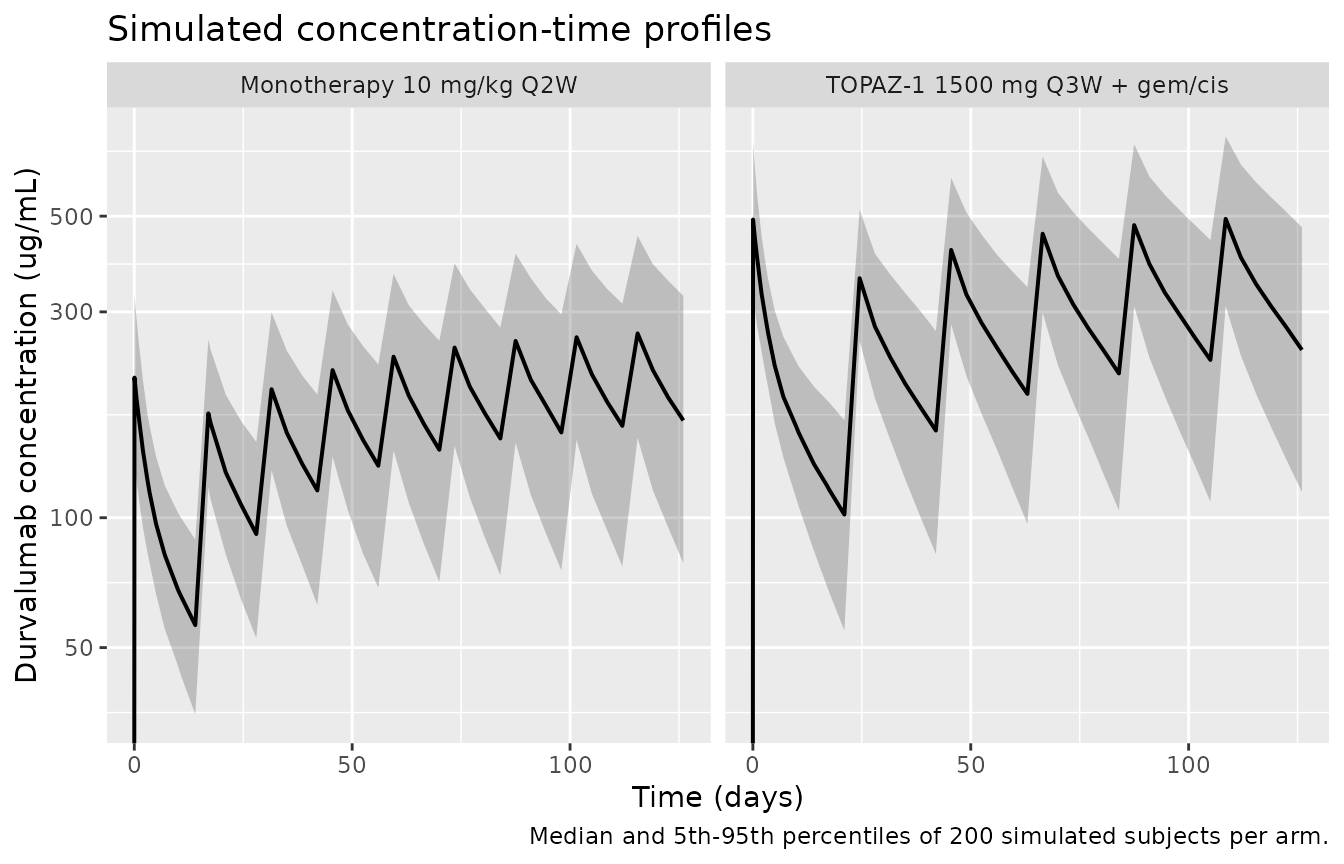
Simulated durvalumab concentration-time profiles by regimen (median with 5th-95th percentile band, n = 200 per arm). Comparable in shape to the pcVPC of Supplementary Fig. S1c.
PKNCA validation
The paper defines AUC 0-21d as “the AUC from day 0 to
day 21 (1st cycle for durvalumab with Gem/Cis), calculated using the
linear up/log down variant of the trapezoidal rule”, and
Cmin1 as “the minimum durvalumab concentration at day 21”.
PKNCA is configured to match:
auc.method = "lin up/log down", and the day-21 value is
taken as ctrough, which reads the record sitting exactly on
the interval end rather than the minimum over the interval.
Cycle-1 metrics are computed on a single-dose
simulation so that no dose falls on the interval end – a dose exactly at
end makes PKNCA report the following peak as
cmax.
PKNCA::PKNCA.options(auc.method = "lin up/log down")

events_sd <- events |>
  filter(time <= 21) |>
  filter(!(evid == 1 & time > 0))

sim_sd <- rxode2::rxSolve(mod, events = events_sd, keep = "regimen") |>
  as.data.frame()

conc_sd <- sim_sd |>
  # Only !is.na(): a `time > 0` or `Cc > 0` filter would drop the time-zero
  # row that PKNCA needs to anchor AUC0-*. The solve output has no evid
  # column and already contains only observation rows.
  filter(!is.na(Cc)) |>
  select(id, time, Cc, regimen)

# The time-zero record PKNCA needs must actually be present.
stopifnot(all(tapply(conc_sd$time, conc_sd$id, min) == 0))
stopifnot(all(tapply(conc_sd$time, conc_sd$id, max) == 21))

conc_obj <- PKNCA::PKNCAconc(conc_sd, Cc ~ time | regimen + id)

dose_sd <- events_sd |>
  filter(evid == 1) |>
  select(id, time, amt, regimen)

dose_obj <- PKNCA::PKNCAdose(dose_sd, amt ~ time | regimen + id)

intervals <- data.frame(
  start   = 0,
  end     = 21,
  cmax    = TRUE,
  tmax    = TRUE,
  auclast = TRUE,
  ctrough = TRUE
)

nca_res <- PKNCA::pk.nca(PKNCA::PKNCAdata(conc_obj, dose_obj, intervals = intervals))

nca_summary <- as.data.frame(nca_res) |>
  group_by(regimen, PPTESTCD) |>
  summarise(
    Median = stats::median(PPORRES, na.rm = TRUE),
    P25    = stats::quantile(PPORRES, 0.25, na.rm = TRUE),
    P75    = stats::quantile(PPORRES, 0.75, na.rm = TRUE),
    .groups = "drop"
  )

nca_summary |>
  dplyr::rename(
    "Regimen"        = regimen,
    "NCA parameter"  = PPTESTCD,
    "Median"         = Median,
    "25th pct"       = P25,
    "75th pct"       = P75
  ) |>
  knitr::kable(
    digits  = 2,
    caption = "Simulated cycle-1 NCA after a single durvalumab dose (n = 200 per arm). Cmax and Ctrough in ug/mL, AUClast in ug*day/mL, Tmax in days -- Tmax is the end of the 1 h infusion, 1/24 = 0.04 days, for every subject in an intravenous model."
)| Regimen | NCA parameter | Median | 25th pct | 75th pct |
|---|---|---|---|---|
| Monotherapy 10 mg/kg Q2W | auclast | 1709.87 | 1452.04 | 1994.51 |
| Monotherapy 10 mg/kg Q2W | cmax | 210.87 | 178.56 | 246.69 |
| Monotherapy 10 mg/kg Q2W | ctrough | 42.94 | 34.43 | 52.13 |
| Monotherapy 10 mg/kg Q2W | tmax | 0.04 | 0.04 | 0.04 |
| TOPAZ-1 1500 mg Q3W + gem/cis | auclast | 3960.20 | 3486.69 | 4573.38 |
| TOPAZ-1 1500 mg Q3W + gem/cis | cmax | 517.49 | 411.47 | 601.70 |
| TOPAZ-1 1500 mg Q3W + gem/cis | ctrough | 97.77 | 82.32 | 122.90 |
| TOPAZ-1 1500 mg Q3W + gem/cis | tmax | 0.04 | 0.04 | 0.04 |
# A shape check, not a published comparison: every subject must have a finite
# cycle-1 Cmax and trough, or a later comparison would silently run on NAs.
stopifnot(all(is.finite(nca_summary$Median)))
stopifnot(nrow(nca_summary) == 8L)
Comparison against published NCA
Supplementary Table S1 reports the model-predicted dose-1 trough
(Cmin, dose 1) for all 314 TOPAZ-1 durvalumab-arm patients,
split into exposure quartiles. The quartile boundaries pin the
cohort quantiles tightly, because each quartile’s maximum and the next
quartile’s minimum bracket the boundary:
| Quantile | Bracketing values from Table S1 | Target |
|---|---|---|
| 25th percentile | Q1 max 79.0, Q2 min 79.1 | 79.05 ug/mL |
| Median | Q2 max 94.1, Q3 min 95.1 | 94.6 ug/mL |
| 75th percentile | Q3 max 113, Q4 min 113 | 113 ug/mL |
topaz_ctrough <- as.data.frame(nca_res) |>
  filter(regimen == "TOPAZ-1 1500 mg Q3W + gem/cis", PPTESTCD == "ctrough") |>
  pull(PPORRES)

published_cmin1d <- c(P25 = 79.05, Median = 94.6, P75 = 113)
simulated_cmin1d <- stats::quantile(topaz_ctrough, c(0.25, 0.5, 0.75))

cmin_cmp <- tibble::tibble(
  Quantile     = names(published_cmin1d),
  `Published (ug/mL)` = as.numeric(published_cmin1d),
  `Simulated (ug/mL)` = as.numeric(simulated_cmin1d)
) |>
  mutate(`Difference (%)` = 100 * (`Simulated (ug/mL)` / `Published (ug/mL)` - 1))

knitr::kable(
  cmin_cmp,
  digits  = 1,
  caption = "Dose-1 trough (day 21) in the TOPAZ-1 arm: simulated cohort versus the quartile boundaries of Supplementary Table S1."
)| Quantile | Published (ug/mL) | Simulated (ug/mL) | Difference (%) |
|---|---|---|---|
| P25 | 79.0 | 82.3 | 4.1 |
| Median | 94.6 | 97.8 | 3.4 |
| P75 | 113.0 | 122.9 | 8.8 |
The single combined comparison table required for the published-NCA
check uses the same numbers through ncaComparisonTable(),
which joins on the regimen and reports the median:
published <- tibble::tibble(
  regimen = "TOPAZ-1 1500 mg Q3W + gem/cis",
  ctrough = 94.6
)

cmp <- nlmixr2lib::ncaComparisonTable(
  simulated     = nca_res,
  reference     = published,
  by            = "regimen",
  units         = c(ctrough = "ug/mL"),
  tolerance_pct = 20
)

knitr::kable(
  cmp,
  caption = "Simulated vs. published dose-1 trough. * differs from reference by >20%.",
  align   = c("l", "l", "r", "r", "r")
)| NCA parameter | regimen | Reference | Simulated | % diff |
|---|---|---|---|---|
| Ctrough (ug/mL) | TOPAZ-1 1500 mg Q3W + gem/cis | 94.6 | 97.8 | +3.4% |
pct_diff <- cmin_cmp$`Difference (%)`

# Centre: a mis-transcribed clearance, volume, dose or unit moves the whole
# distribution by tens of percent, so the median is the load-bearing check.
# Measured while authoring: the median difference was +7.1% at each of 1, 2,
# 4, 8 and 16 solver threads for a 200-subject single-arm draw, and +7.3% for
# the 400-subject two-arm draw this vignette actually renders (a different
# eta draw, not a different model). 15 sits outside that spread while still
# going red for a real transcription error -- raising CL from 0.298 to 0.398
# L/day, for instance, drops the day-21 trough by about a third.
stopifnot(abs(pct_diff[cmin_cmp$Quantile == "Median"]) < 15)

# Envelope: the quartiles depend on which subjects were drawn, and the
# published spread additionally reflects EBE shrinkage that a forward
# simulation does not reproduce, so these get more room than the median.
# Measured max |difference| across the same runs: 12.6% (P75, 200-subject
# draw) and 10.2% (P75, the 400-subject draw rendered here).
stopifnot(max(abs(pct_diff)) < 25)
The simulated cohort reproduces the published dose-1 trough distribution to within a few percent at the median. The interquartile spread is expected to be slightly wider in simulation than in the published summary: the published values are individual empirical Bayes predictions, which are shrunk toward the typical value (Table 4 reports 19.1% shrinkage on CL and 25.7% on V1), whereas the forward simulation draws unshrunken etas.
ggplot(tibble::tibble(ctrough = topaz_ctrough), aes(ctrough)) +
  geom_histogram(bins = 30, fill = "grey70", colour = "white") +
  geom_vline(xintercept = published_cmin1d, linetype = "dashed") +
  labs(
    x = "Dose-1 trough at day 21 (ug/mL)", y = "Subjects",
    title = "Dose-1 trough, TOPAZ-1 arm",
    caption = "Dashed: 25th / 50th / 75th percentiles from Supplementary Table S1."
  )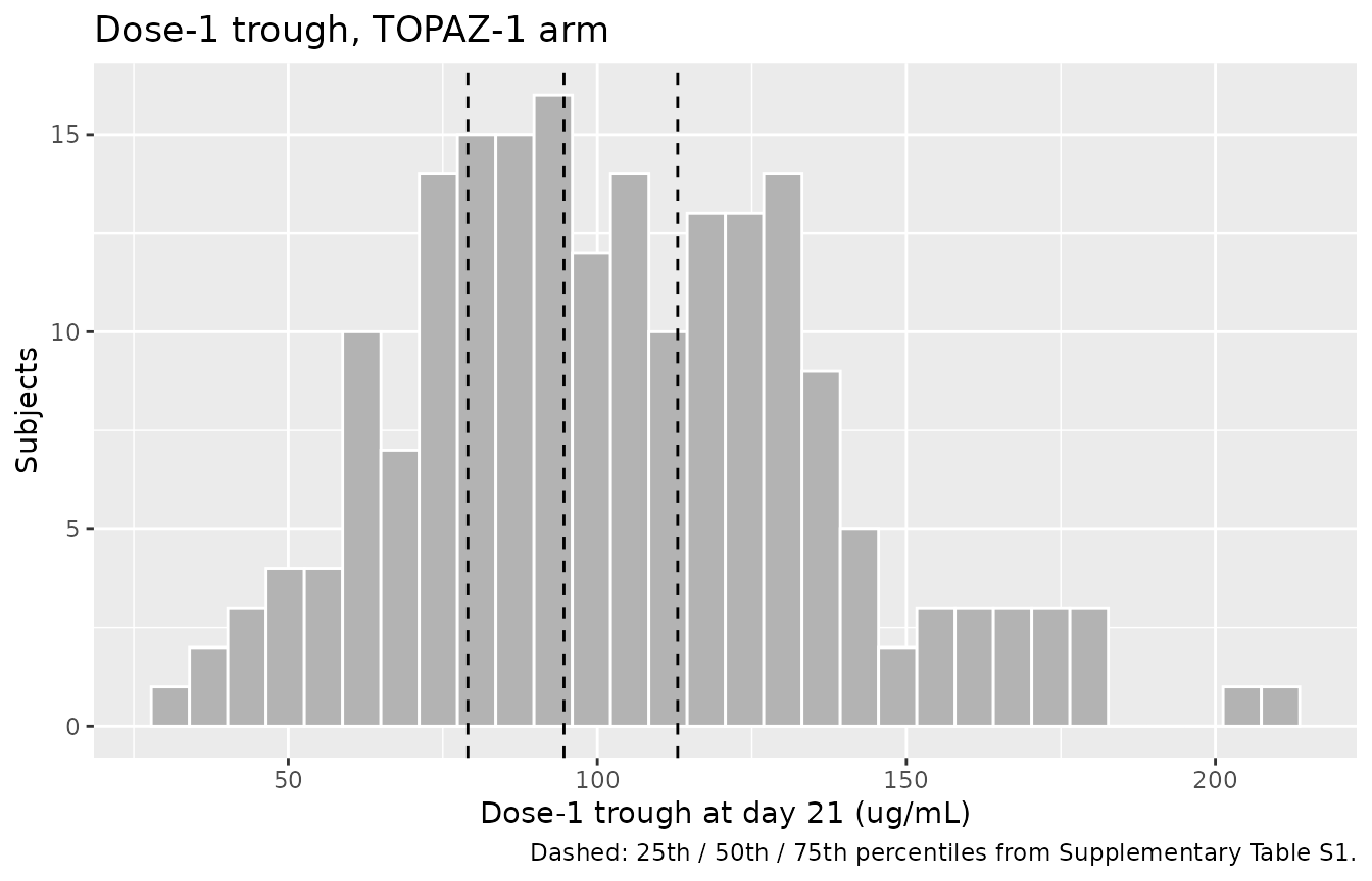
Simulated dose-1 trough distribution in the TOPAZ-1 arm. Vertical lines are the quartile boundaries derived from Supplementary Table S1.
Steady-state accumulation
The paper computes Cmax,ss and AUCss after
“achieving steady state (16 weeks)” but publishes no numeric values for
them, so this is a self-consistency check rather than a reproduction:
with a time-dependent clearance that falls towards 61% of baseline,
accumulation over 18 weeks must exceed what a time-invariant model would
give.
topaz_sim <- sim_all |> filter(regimen == "TOPAZ-1 1500 mg Q3W + gem/cis")

trough_cycle1 <- topaz_sim |> filter(time == 21) |> pull(Cc)
trough_late   <- topaz_sim |> filter(time == 126) |> pull(Cc)

accumulation <- stats::median(trough_late) / stats::median(trough_cycle1)
accumulation
#> [1] 2.412758

# Q3W dosing with a ~14 day terminal half-life accumulates roughly 2-fold even
# without the time-varying term; the falling clearance pushes it higher. The
# bound is a direction-and-magnitude check, not a published number.
stopifnot(accumulation > 1.5, accumulation < 4)
Assumptions and deviations
-
IIV on the time-varying-clearance asymptote is additive, not
log-normal. Abegesah 2025 reports
ETA Tmax= 0.0623 in Table 4 but printsexp(eta_i)only on clearance itself, and never states the form of the Tmax random effect. The additive formTmax_i = Tmax + etais taken from the sibling AstraZeneca modelHwang_2022_tremelimumab.R– the same modelling group, the same senior author, and the sameTmax * t^lambda / (TC50^lambda + t^lambda)parameterization – where it is verified against the published NONMEM control stream. Becausecl_time_maxis negative (-0.498), a log-normal form is not available anyway. Under the additive form roughly 2% of subjects draw an eta large enough to flip the sign and show a rising clearance; the same is true, more strongly, of the Hwang model. -
IIV on V1 is exponential. The printed
Vc,iequation on page 3 shows no random-effect term, but Table 4 reportsETA V1= 0.0593 together with aCov CL-V1off-diagonal, and the Methods state the CL-V1 correlation was “estimated via omega block”. The standard exponential form is used, matching the clearance equation that the paper does print in full. -
LAMis treated as fixed. Table 4 reports 1.00 with no RSE, no bootstrap median and no confidence interval – the signature of a fixed parameter – and atLAM= 1 the general Hill form collapses exactly to theexp(Tmax * t / (TC50 + t))expression the paper prints. - Residual-error estimates are read as standard deviations. Table 4’s Bootstrap-median column reports 0.0649 and 23.0 for the two residual rows, which are the squares of the Estimate column’s 0.255 and 4.75, while the 95% CI column ([0.246; 0.263] and [3.55; 6.17]) stays on the same scale as the Estimate. One column of that table slipped to the variance scale; the Estimate and CI columns agree with each other and are used.
-
The three time-varying-clearance parameters are not
log-transformed.
checkModelConventions()suggestslcl_time_max/lcl_t50/lcl_time_hill.cl_time_maxis negative and cannot be log-transformed, and the other two are kept on the linear scale so the model is directly comparable withHwang_2022_tremelimumab.R, which carries the identical warning forcl_t50.cl_time_max,cl_t50andcl_time_hillare the canonical names for this family ininst/references/parameter-names.md. - Covariate distributions are assumed. Table 2 publishes only medians and ranges for the continuous covariates. Body-weight dispersion (CV 24%) and albumin dispersion (SD 4.8 g/L) are pooled from the durvalumab-arm quartile means and SDs of Supplementary Table S1; creatinine clearance and LDH dispersions are chosen so the drawn 5th-95th range is consistent with the published min-max, and are documented here because the paper does not report them. LDH carries an exponent of 0.0515, so its assumed spread has almost no influence on the results.
-
Race is not a model covariate. The Results state
that “the influence of age and race was not significant”, and no
coefficient is reported for either, so neither appears in
model(). Both are recorded incovariatesDataExcludedfor provenance. -
The exposure-response models are not packaged. The
overall-survival analysis is a Cox proportional hazards model (Table 3:
logNLR 0.678, logALB -2.258, disease status -0.900) whose baseline
hazard
h0(t)is not reported, so it cannot be simulated. The safety analyses found no exposure-response relationship and consequently report no fitted logistic-regression coefficients – Fig. 3 shows the exploratory plots only. Neither analysis yields a parameterized, simulatable sub-model. - No time-varying covariates. All covariates are treated as baseline values held constant over the simulation, as the paper’s “baseline” covariate definitions imply.
Errata and internal inconsistencies in the source
Three places where Abegesah 2025 contradicts itself. In each case the
resolution and its justification are recorded here and in the model
file’s covariateData notes.
The Table 4 legend mislabels COMB1. The legend glosses “Comb1” as “durvalumab and tremelimumab without chemotherapy”. Two of the paper’s own data sources say otherwise: Fig. 1 labels the -16.3% bar (which is the COMB1 estimate of -0.163) “Combo Durva + Chemo”, and Table 2 assigns all 314 TOPAZ-1 patients – who received durvalumab with gemcitabine/cisplatin and no tremelimumab – to the second of the three combination levels. COMB1 is therefore read as durvalumab + chemotherapy, and COMB2, whose legend entry (“durvalumab, tremelimumab and chemotherapy”) is corroborated by the Fig. 1 bar “Combo Durva + Treme + Chemo”, is read as printed.
-
The tumor-type-1 coefficient has conflicting signs. Table 4 prints “Tumor type 1 on CL” as +0.0101; the page 3
CL_cat.covequation prints(1 - 0.0101). Every other categorical factor in that equation equals(1 + theta)using the signed Table 4 estimate, so this one term breaks the pattern. The equation is followed, per the standing text-versus-equation convention. Nothing turns on the choice: the estimate has an RSE of 185% and a bootstrap 95% CI of [-0.0228; 0.0466] spanning zero, so a 1% effect of either sign is indistinguishable from none.The same stratum is also never labelled. Table 4 names it only “Tumor type 1”, and unlike the level-2 and level-3 bars (“TUM TYP Bladder”, “TUM TYP BTC”) it is absent from Fig. 1 altogether. It is stored under the register’s residual
TUMTP_OTHERcolumn, with its composition inferred as the non-NSCLC / non-bladder / non-BTC remainder – small-cell lung cancer plus the miscellaneous Study 1108 advanced solid tumours. The Fig. 1 ECOG bar points the wrong way. Fig. 1 draws “ECOG restricted activity” as +5.3%, a clearance increase. Both of the paper’s other statements of that effect disagree: Table 4 gives -0.0501 and the page 3
CL_cat.covequation prints(1 - 0.0501), i.e. a 5.0% decrease. The equation and table are followed. The negative direction is independently corroborated by the upstream Baverel 2018 durvalumab model, transcribed in the siblingdeVries_2025_durvalumab.Ras0.937^ECOG_GE1– a 6.3% lower clearance for ECOG >= 1. Note that +5.3% is almost exactly1 / (1 - 0.0501) - 1= +5.27%, consistent with that one bar having been plotted as the inverse ratio. This is why the ECOG bar is checked separately from the Fig. 1 tornado table above.