Posaconazole (Winchell 2024)
Source:vignettes/articles/Winchell_2024_posaconazole.Rmd
Winchell_2024_posaconazole.RmdModel and source
mod <- rxode2::rxode2(nlmixr2lib::readModelDb("Winchell_2024_posaconazole"))
#> ℹ parameter labels from comments will be replaced by 'label()'- Citation: Winchell G, de Greef R, Ouerdani A, Fauchet F, Wrishko RE, Mangin E, Bruno C, Waskin H. A population pharmacokinetic model for posaconazole intravenous solution and oral powder for suspension formulations in pediatric patients with neutropenia. Antimicrob Agents Chemother. 2024;68(4):e01197-23. doi:10.1128/aac.01197-23.
- Article: https://doi.org/10.1128/aac.01197-23
- Supplement (Tables S1-S3, Fig. S1-S4): https://doi.org/10.1128/aac.01197-23 (file
aac.01197-23-s0001.pdf; also available with the open-access record, PMC10994819)
Winchell 2024 is the pediatric companion to the adult posaconazole
tablet population PK analysis of the same group, which is also packaged
here as vanIersel_2018_posaconazole
and is cited as reference 18 of the present paper (“A one-compartment
model with first-order absorption was fit to the PK data set … based on
the previous analyses of posaconazole PK in adults”).
Population
The analysis data set comprised 1,236 plasma posaconazole observations from 114 immunocompromised pediatric participants aged 2 to 17 years with documented or anticipated neutropenia, enrolled in the phase 1b open-label sequential dose-escalation study P097 (MK-5592-097, ClinicalTrials.gov NCT02452034). Baseline characteristics are Winchell 2024 Table 1: median age 8 years (range 2-17), median body weight 28.6 kg (range 10.2-102), median eGFR 146 mL/min/1.73 m^2 (range 12.2-314). About 59% were male, 83% White and 87% not Hispanic. Participants received 3.5 (n = 35), 4.5 (n = 31), or 6 mg/kg (n = 48) posaconazole – IV BID on day 1, IV QD on days 2-10, then either oral PFS (n = 60) or IV (n = 54) QD on days 10-28 – with the absolute dose capped at 300 mg. Eighty samples were excluded (33 from two participants with incomplete oral PFS dose intakes, 31 with no sampling time, 13 with a duplicate sampling time), and concentrations below the 5.00 ng/mL LLOQ were excluded rather than modelled.
The two age strata that the paper simulates separately are 2 to <7 years (n = 48, median weight 16 kg, range 10.2-41.7) and 7 to 17 years (n = 66, median weight 45.4 kg, range 18.2-102).
The same information is available programmatically:
str(nlmixr2lib::readModelDb("Winchell_2024_posaconazole")()$population)
#> List of 13
#>  $ species       : chr "human"
#>  $ n_subjects    : int 114
#>  $ n_studies     : int 1
#>  $ n_observations: chr "1,236 plasma posaconazole PK observations (Winchell 2024 Results 'Participant characteristics'). 80 samples wer"| __truncated__
#>  $ age_range     : chr "2-17 years (median 8; 2-<7 years subgroup median 3, 7-17 years subgroup median 13)"
#>  $ weight_range  : chr "10.2-102 kg (median 28.6; 2-<7 years subgroup median 16, range 10.2-41.7; 7-17 years subgroup median 45.4, range 18.2-102)"
#>  $ sex_female_pct: num 41
#>  $ race_ethnicity: chr "83% White; 87% not Hispanic (Winchell 2024 Results 'Participant characteristics')"
#>  $ disease_state : chr "Immunocompromised pediatric patients aged 2 to 17 years with documented or anticipated neutropenia in the setti"| __truncated__
#>  $ dose_range    : chr "3.5, 4.5, or 6 mg/kg posaconazole, IV BID on day 1 then IV QD on days 2-10, followed by either oral PFS or IV Q"| __truncated__
#>  $ regions       : chr "Not reported (multicenter phase 1b study P097 / MK-5592-097, ClinicalTrials.gov NCT02452034)"
#>  $ renal_function: chr "Median eGFR 146 mL/min/1.73 m2 (range 12.2-314); eGFR was screened as a covariate and not retained."
#>  $ notes         : chr "Fit in NONMEM 7.2 with FOCE and an additive residual-error model on log-transformed concentrations. Observation"| __truncated__
Source trace
| Equation / parameter | Value | Source location |
|---|---|---|
One compartment, first-order absorption, IV into
central
|
structure | Results “Final model”; Methods “Population PK model development” (“with IV administration being assumed to be directed into the central compartment”) |
lcl (CL) |
4.71 L/h (RSE 3.86%) | Table 2, “CL (L/h)” |
lvc (Vc) |
112 L (RSE 5.18%) | Table 2, “Vc (L)” |
lka (ka) |
0.212 1/h (RSE 17.9%) | Table 2, “KA (h-1)” |
logitfdepot (F1) |
0.826 (RSE 5.58%), on the logit scale | Table 2, “F1”; Results “Final model” (“estimated bioavailability using a logit function (in order to constrain its value between 0 and 1)”) |
e_wt_cl |
0.624 (RSE 9.86%), estimated | Table 2, “alpha for CL”; Results “Final model” |
e_wt_vc |
0.971 (RSE 7.86%), estimated | Table 2, “alpha for Vc”; Results “Final model” |
etalcl variance |
0.371^2 = 0.137641 | Table 2, “IIV (CL)” = 37.1 with footnote b (“a CV%, calculated by the square root of Omega, multiplied by 100”) |
etalvc variance |
0.277^2 = 0.076729 | Table 2, “IIV (Vc)” = 27.7 with footnote b |
etalcl-etalvc covariance |
not reported; set to 0 | Results “Final model” states a correlation between CL and Vc exists but no magnitude is given anywhere in the paper or supplement |
etalogitfdepot variance |
2.02^2 = 4.0804 | Table 2, “IIV (F1)” = 2.02 with footnote c (“shown as a standard deviation in the logit domain … 95% of patients having F1 comprising between 8% and 99%”) |
expSd |
0.331 (RSE 4.71%) | Table 2, “Residual error, SD”; Results “Final model” (“an additive error model in the logarithmic scale”) |
| Allometric reference weight | 28.6 kg | Table 1, “All (N = 114)” median weight. Not stated by the paper as the covariate-model reference – see Assumptions and deviations |
| No covariate retained (age, weight, eGFR, sex, ethnicity) | – | Results “Final model” (“therefore, the base structural model was considered the final model”) |
| No food effect on bioavailability | – | Results “Effect of food”; Fig. 1 |
Exact structural checks
These four checks are independent of any assumption about the
simulated cohort, so they test the packaged model itself rather than the
virtual population. Each is a hard stopifnot().
The logit-domain bioavailability SD reproduces the paper’s own F1 interval
Table 2 footnote c states that the F1 variability of 2.02 “corresponds to 95% of patients having F1 comprising between 8% and 99%”. That sentence is what fixes 2.02 as a standard deviation (not a variance) in the logit domain: reading it as a variance would give a 95% interval of 23% to 99%.
ini_tbl <- mod$iniDf
# Fixed effects carry ntheta; random-effect variances carry neta1 == neta2.
logitf1 <- ini_tbl$est[!is.na(ini_tbl$ntheta) & ini_tbl$name == "logitfdepot"]
om_f1 <- sqrt(ini_tbl$est[!is.na(ini_tbl$neta1) &
                            ini_tbl$neta1 == ini_tbl$neta2 &
                            ini_tbl$name == "etalogitfdepot"])
stopifnot(length(logitf1) == 1, length(om_f1) == 1)
c(logitfdepot = logitf1, sd_logit_F1 = om_f1)
#> logitfdepot sd_logit_F1
#>    1.557539    2.020000

f1_ci <- plogis(logitf1 + c(-1.96, 1.96) * om_f1)
# The alternative reading, in which the tabulated 2.02 were a variance rather
# than an SD, so the logit-domain SD would be sqrt(2.02) = 1.42.
f1_ci_var <- plogis(logitf1 + c(-1.96, 1.96) * sqrt(om_f1))

rbind(`2.02 as logit-domain SD` = 100 * f1_ci,
      `2.02 as logit-domain variance` = 100 * f1_ci_var) |>
  round(1)
#>                               [,1] [,2]
#> 2.02 as logit-domain SD        8.3 99.6
#> 2.02 as logit-domain variance 22.7 98.7

# Paper footnote c states "between 8% and 99%". The lower bound is what
# discriminates the two readings: the SD reading gives 8%, the variance
# reading gives 23%. The upper bound is 99.6%, which the paper reports
# truncated to 99%.
stopifnot(
  abs(100 * f1_ci[1] - 8) < 0.5,
  100 * f1_ci[2] >= 99, 100 * f1_ci[2] < 100,
  100 * f1_ci_var[1] > 20            # the variance reading is refuted
)
Allometric scaling, dose proportionality, and the Cavg identity
At steady state a one-compartment linear model must satisfy
Cavg = Dose * F / (CL * tau) exactly, and clearance must
scale as (WT / 28.6)^0.624. Both are checked against a
typical-value (no-IIV) simulation of the final QD dosing interval.
omega = NA suppresses the random effects without mutating
the shared model object.
tau <- 24

# Average concentration over a dosing interval by the trapezoidal rule. A plain
# mean() of grid points is biased for the IV arms, where the bolus makes C(0+)
# the peak and C(tau-) the trough.
trap_mean <- function(time, conc) {
  sum(diff(time) * (head(conc, -1) + tail(conc, -1)) / 2) /
    (max(time) - min(time))
}

typ_events <- bind_rows(
  # IV dose straight into central; PFS dose into depot.
  data.frame(id = 1:4, time = 0, amt = c(100, 100, 300, 300),
             cmt = rep(c("central", "depot"), each = 2),
             evid = 1L, ii = tau, ss = 1L, WT = c(20, 60, 20, 60)),
  expand.grid(id = 1:4, time = seq(0, tau, by = 0.1)) |>
    mutate(amt = 0, cmt = "central", evid = 0L, ii = 0, ss = 0L,
           WT = c(20, 60, 20, 60)[id])
) |>
  arrange(id, time, -evid)

typ <- rxode2::rxSolve(mod, typ_events, omega = NA, returnType = "data.frame",
                       keep = "WT",
                       # steady-state searches for long-half-life subjects exceed the default step budget
                       maxsteps = 1e6) |>
  filter(!is.na(Cc))
#> Warning: multi-subject simulation without without 'omega'

# Allometric identity on CL and Vc.
cl_wt <- typ |> group_by(WT) |> summarise(cl = first(cl), vc = first(vc), .groups = "drop")
stopifnot(
  isTRUE(all.equal(cl_wt$cl[cl_wt$WT == 60] / cl_wt$cl[cl_wt$WT == 20],
                   (60 / 20)^0.624, tolerance = 1e-8)),
  isTRUE(all.equal(cl_wt$vc[cl_wt$WT == 60] / cl_wt$vc[cl_wt$WT == 20],
                   (60 / 20)^0.971, tolerance = 1e-8))
)

# Cavg = Dose * F / (CL * tau).  F = 1 for the IV rows, F1 for the PFS rows.
f1_typ <- plogis(logitf1)
cavg_check <- typ |>
  group_by(id, WT) |>
  summarise(cavg_sim = trap_mean(time, Cc), cl = first(cl),
            fdepot = first(fdepot), .groups = "drop") |>
  mutate(route = c("IV", "IV", "PFS", "PFS"),
         amt = c(100, 100, 300, 300),
         f = ifelse(route == "IV", 1, fdepot),
         cavg_closed = amt * f / (cl * tau) * 1000,
         pct = 100 * (cavg_sim / cavg_closed - 1))
cavg_check |> select(route, WT, amt, cavg_sim, cavg_closed, pct)
#> # A tibble: 4 × 6
#>   route    WT   amt cavg_sim cavg_closed       pct
#>   <chr> <dbl> <dbl>    <dbl>       <dbl>     <dbl>
#> 1 IV       20   100    1106.       1106.  0.000223
#> 2 IV       60   100     557.        557.  0.000144
#> 3 PFS      20   300    2740.       2740. -0.000845
#> 4 PFS      60   300    1381.       1381. -0.000594

stopifnot(all(abs(cavg_check$pct) < 0.01))
stopifnot(isTRUE(all.equal(unname(f1_typ), 0.826, tolerance = 1e-3)))
Dose proportionality of the IV arm (uncapped) is then exact by construction:
prop_events <- bind_rows(
  data.frame(id = 1:2, time = 0, amt = c(4.5, 6) * 25, cmt = "central",
             evid = 1L, ii = tau, ss = 1L, WT = 25),
  expand.grid(id = 1:2, time = seq(0, tau, by = 0.1)) |>
    mutate(amt = 0, cmt = "central", evid = 0L, ii = 0, ss = 0L, WT = 25)
) |>
  arrange(id, time, -evid)

prop <- rxode2::rxSolve(mod, prop_events, omega = NA, returnType = "data.frame",
                        # steady-state searches for long-half-life subjects exceed the default step budget
                        maxsteps = 1e6) |>
  filter(!is.na(Cc)) |>
  group_by(id) |>
  summarise(cavg = trap_mean(time, Cc), .groups = "drop")
#> Warning: multi-subject simulation without without 'omega'

ratio <- prop$cavg[2] / prop$cavg[1]
c(observed = ratio, expected = 6 / 4.5)
#> observed expected
#> 1.333333 1.333333
stopifnot(isTRUE(all.equal(ratio, 6 / 4.5, tolerance = 1e-6)))
Virtual cohort
The paper’s simulations drew 1,000 subjects per age stratum by jointly sampling age and weight from the pooled P097 and P032 pediatric populations. That pooled weight distribution is not reported, so the cohort here is reconstructed from the only weight information the paper publishes – the per-stratum median and range of Winchell 2024 Table 1 – as a log-normal whose median matches the reported median and whose 0.5th/99.5th percentiles span the reported range. Weights are taken at deterministic quantiles rather than random draws so the comparison below is reproducible and free of sampling artifacts.
The random effects are likewise assigned at deterministic quantiles, as a Latin hypercube: each eta’s marginal distribution is reproduced exactly (up to the quantile grid), and the same subject-level draws are reused across every dose and formulation arm. This is the common-random-numbers device – it makes the between-arm contrasts exact rather than Monte Carlo estimates, so the PFS/IV comparison below isolates bioavailability instead of mixing in sampling noise.
n_per_group <- 200

make_weights <- function(median_wt, lo, hi, n) {
  # log-normal matched to the reported median and range (range ~ +/- 2.576 SD)
  sdlog <- (log(hi) - log(lo)) / (2 * 2.576)
  q <- qlnorm(seq(0.5, n - 0.5) / n, meanlog = log(median_wt), sdlog = sdlog)
  pmin(pmax(q, lo), hi)
}

# Latin-hypercube eta draws: exact marginals, fixed permutation per eta.
lhs_normal <- function(n, sd, seed) {
  set.seed(seed)
  sd * qnorm((sample.int(n) - 0.5) / n)
}

om <- c(etalcl = sqrt(0.137641), etalvc = sqrt(0.076729),
        etalogitfdepot = 2.02)

make_subjects <- function(agegrp, median_wt, lo, hi, seed0) {
  data.frame(
    agegrp = agegrp,
    WT = make_weights(median_wt, lo, hi, n_per_group),
    etalcl = lhs_normal(n_per_group, om[["etalcl"]], seed0 + 1L),
    etalvc = lhs_normal(n_per_group, om[["etalvc"]], seed0 + 2L),
    etalogitfdepot = lhs_normal(n_per_group, om[["etalogitfdepot"]], seed0 + 3L)
  )
}

cohort <- bind_rows(
  make_subjects("2 to <7 years", 16, 10.2, 41.7, 100L),
  make_subjects("7 to 17 years", 45.4, 18.2, 102, 200L)
)

cohort |>
  group_by(agegrp) |>
  summarise(n = n(), median_wt = median(WT), min_wt = min(WT), max_wt = max(WT),
            geomean_wt = exp(mean(log(WT))), .groups = "drop")
#> # A tibble: 2 × 6
#>   agegrp            n median_wt min_wt max_wt geomean_wt
#>   <chr>         <int>     <dbl>  <dbl>  <dbl>      <dbl>
#> 1 2 to <7 years   200      16.0   10.2   34.5       16.1
#> 2 7 to 17 years   200      45.4   18.2  102         45.4
The cohort’s realised relative bioavailability distribution matches the analytic logit-normal, including the geometric mean that drives the PFS/IV contrast:
f1_cohort <- plogis(logitf1 + cohort$etalogitfdepot)
gm_f1_cohort <- exp(mean(log(f1_cohort)))
c(cohort_GM_F1 = gm_f1_cohort,
  cohort_p2.5 = unname(quantile(f1_cohort, 0.025)),
  cohort_p97.5 = unname(quantile(f1_cohort, 0.975)))
#> cohort_GM_F1  cohort_p2.5 cohort_p97.5
#>   0.62417113   0.08926585   0.99566918
Simulation of the final steady-state dosing interval
Winchell 2024 computed Cavg and Cmin “after the last dose of IV and
PFS administration” on day 28 of QD dosing. Eighteen days of QD dosing
is far beyond steady state for a drug with a 16.5 h typical half-life,
so the final interval is simulated directly with ss = 1 and
ii = 24, which is exact rather than approximate. IV arms
dose into central; PFS arms dose into depot,
where the logit-scale relative bioavailability applies. The 300 mg
absolute cap is imposed as in the paper.
arms <- expand.grid(dose_mgkg = c(4.5, 6, 7.5), form = c("IV", "PFS"),
                    agegrp = unique(cohort$agegrp),
                    stringsAsFactors = FALSE)

obs_grid <- seq(0, tau, by = 0.5)

eta_cols <- c("etalcl", "etalvc", "etalogitfdepot")

events <- lapply(seq_len(nrow(arms)), function(k) {
  a <- arms[k, ]
  # Same subjects (weights AND etas) in every arm -- common random numbers.
  s <- cohort[cohort$agegrp == a$agegrp, ]
  # Distinct id blocks per arm: rxode2 keys on `id` alone, so reusing ids
  # across arms would collapse them into single multi-regimen subjects.
  ids <- (k - 1L) * n_per_group + seq_len(nrow(s))
  amt <- pmin(a$dose_mgkg * s$WT, 300)
  rows <- rep(seq_len(nrow(s)), each = length(obs_grid))
  bind_rows(
    cbind(data.frame(id = ids, time = 0, amt = amt,
                     cmt = if (a$form == "IV") "central" else "depot",
                     evid = 1L, ii = tau, ss = 1L, WT = s$WT),
          s[, eta_cols]),
    cbind(data.frame(id = ids[rows],
                     time = rep(obs_grid, times = nrow(s)),
                     amt = 0, cmt = "central", evid = 0L, ii = 0, ss = 0L,
                     WT = s$WT[rows]),
          s[rows, eta_cols])
  ) |>
    mutate(agegrp = a$agegrp, form = a$form, dose_mgkg = a$dose_mgkg)
}) |>
  bind_rows() |>
  arrange(id, time, -evid)

# omega = NA: the etas are supplied per subject from the Latin hypercube above
# rather than resampled internally, so the whole vignette is deterministic.
sim <- rxode2::rxSolve(mod, events, omega = NA, returnType = "data.frame",
                       keep = c("WT", "agegrp", "form", "dose_mgkg"),
                       # steady-state searches for long-half-life subjects exceed the default step budget
                       maxsteps = 1e6) |>
  filter(!is.na(Cc)) |>
  mutate(dose_label = paste0(dose_mgkg, " mg/kg"))
#> Warning: multi-subject simulation without without 'omega'

nrow(sim)
#> [1] 117600
Cc is the individual predicted (IPRED) concentration.
Exposure metrics are taken on that scale because the paper’s Cavg and
Cmin are model-derived exposure summaries, not
residual-error-contaminated observations.
PKNCA validation
conc_obj <- PKNCA::PKNCAconc(
  data = sim,
  formula = Cc ~ time | agegrp + dose_label + form + id,
  concu = "ng/mL", timeu = "h"
)

dose_df <- events |>
  filter(evid == 1L) |>
  mutate(dose_label = paste0(dose_mgkg, " mg/kg")) |>
  select(id, time, amt, agegrp, dose_label, form)

dose_obj <- PKNCA::PKNCAdose(
  data = dose_df,
  formula = amt ~ time | agegrp + dose_label + form + id,
  doseu = "mg"
)

intervals <- data.frame(
  start = 0, end = tau,
  cav = TRUE, cmin = TRUE, cmax = TRUE, tmax = TRUE, auclast = TRUE
)

nca <- PKNCA::pk.nca(PKNCA::PKNCAdata(conc_obj, dose_obj, intervals = intervals))

nca_tbl <- as.data.frame(nca$result) |>
  # PKNCA emits dependency/interval rows; keep only the requested interval.
  filter(start == 0, end == tau, !is.na(PPORRES))

nca_tbl |> count(PPTESTCD)
#>   PPTESTCD    n
#> 1  auclast 2400
#> 2      cav 2400
#> 3     cmax 2400
#> 4     cmin 2400
#> 5     tmax 2400
Per-subject Cavg and Cmin are summarised as geometric means to match the supplement, which reports “Predicted geometric mean Cavg and Cmin”.
sim_summary <- nca_tbl |>
  filter(PPTESTCD %in% c("cav", "cmin")) |>
  group_by(agegrp, dose_label, form, PPTESTCD) |>
  summarise(PPORRES = exp(mean(log(PPORRES))),
            geo_cv = 100 * sqrt(exp(var(log(PPORRES))) - 1), .groups = "drop")

sim_summary |>
  select(-geo_cv) |>
  pivot_wider(names_from = PPTESTCD, values_from = PPORRES) |>
  arrange(agegrp, form, dose_label) |>
  rename("Age group" = agegrp, "Dose" = dose_label, "Formulation" = form,
         "Cavg (ng/mL)" = cav, "Cmin (ng/mL)" = cmin) |>
  knitr::kable(digits = 1,
caption = "Simulated steady-state geometric mean exposure.")| Age group | Dose | Formulation | Cavg (ng/mL) | Cmin (ng/mL) |
|---|---|---|---|---|
| 2 to <7 years | 4.5 mg/kg | IV | 917.1 | 422.3 |
| 2 to <7 years | 6 mg/kg | IV | 1222.8 | 563.1 |
| 2 to <7 years | 7.5 mg/kg | IV | 1528.5 | 703.8 |
| 2 to <7 years | 4.5 mg/kg | PFS | 572.3 | 357.6 |
| 2 to <7 years | 6 mg/kg | PFS | 763.0 | 476.8 |
| 2 to <7 years | 7.5 mg/kg | PFS | 953.8 | 596.1 |
| 7 to 17 years | 4.5 mg/kg | IV | 1327.5 | 782.2 |
| 7 to 17 years | 6 mg/kg | IV | 1650.5 | 972.5 |
| 7 to 17 years | 7.5 mg/kg | IV | 1838.1 | 1083.0 |
| 7 to 17 years | 4.5 mg/kg | PFS | 828.4 | 599.3 |
| 7 to 17 years | 6 mg/kg | PFS | 1030.0 | 745.1 |
| 7 to 17 years | 7.5 mg/kg | PFS | 1147.1 | 829.8 |
Comparison against the published simulation (Supplementary Table 2)
Winchell 2024 Supplementary Table 2 reports predicted geometric mean Cavg and Cmin for every age group / dose / formulation combination. All 24 values are transcribed below.
reference_s2 <- tribble(
  ~agegrp,          ~dose_label,  ~form,  ~cav,    ~cmin,
  "2 to <7 years",  "4.5 mg/kg",  "IV",   1044.94,  515.44,
  "2 to <7 years",  "4.5 mg/kg",  "PFS",   796.61,  504.96,
  "2 to <7 years",  "6 mg/kg",    "IV",   1364.60,  656.24,
  "2 to <7 years",  "6 mg/kg",    "PFS",  1049.68,  654.95,
  "2 to <7 years",  "7.5 mg/kg",  "IV",   1713.79,  830.09,
  "2 to <7 years",  "7.5 mg/kg",  "PFS",  1320.77,  827.78,
  "7 to 17 years",  "4.5 mg/kg",  "IV",   1361.00,  795.48,
  "7 to 17 years",  "4.5 mg/kg",  "PFS",  1041.55,  734.80,
  "7 to 17 years",  "6 mg/kg",    "IV",   1748.46, 1035.21,
  "7 to 17 years",  "6 mg/kg",    "PFS",  1331.39,  947.19,
  "7 to 17 years",  "7.5 mg/kg",  "IV",   2001.55, 1210.21,
  "7 to 17 years",  "7.5 mg/kg",  "PFS",  1546.59, 1114.93
)

cmp <- nlmixr2lib::ncaComparisonTable(
  simulated = sim_summary |> select(agegrp, dose_label, form, PPTESTCD, PPORRES),
  reference = reference_s2,
  by = c("agegrp", "dose_label", "form"),
  params = c("cav", "cmin"),
  units = c(cav = "ng/mL", cmin = "ng/mL")
)
cmp |>
  rename("Age group" = agegrp, "Dose" = dose_label, "Formulation" = form) |>
  knitr::kable(digits = 1,
caption = "Simulated vs. Winchell 2024 Supplementary Table 2.")| NCA parameter | Age group | Dose | Formulation | Reference | Simulated | % diff |
|---|---|---|---|---|---|---|
| Cmin (ng/mL) | 2 to <7 years | 4.5 mg/kg | IV | 515 | 422 | -18.1% |
| Cmin (ng/mL) | 2 to <7 years | 4.5 mg/kg | PFS | 505 | 358 | -29.2%* |
| Cmin (ng/mL) | 2 to <7 years | 6 mg/kg | IV | 656 | 563 | -14.2% |
| Cmin (ng/mL) | 2 to <7 years | 6 mg/kg | PFS | 655 | 477 | -27.2%* |
| Cmin (ng/mL) | 2 to <7 years | 7.5 mg/kg | IV | 830 | 704 | -15.2% |
| Cmin (ng/mL) | 2 to <7 years | 7.5 mg/kg | PFS | 828 | 596 | -28.0%* |
| Cmin (ng/mL) | 7 to 17 years | 4.5 mg/kg | IV | 795 | 782 | -1.7% |
| Cmin (ng/mL) | 7 to 17 years | 4.5 mg/kg | PFS | 735 | 599 | -18.4% |
| Cmin (ng/mL) | 7 to 17 years | 6 mg/kg | IV | 1040 | 972 | -6.1% |
| Cmin (ng/mL) | 7 to 17 years | 6 mg/kg | PFS | 947 | 745 | -21.3%* |
| Cmin (ng/mL) | 7 to 17 years | 7.5 mg/kg | IV | 1210 | 1080 | -10.5% |
| Cmin (ng/mL) | 7 to 17 years | 7.5 mg/kg | PFS | 1110 | 830 | -25.6%* |
| Cavg (ng/mL) | 2 to <7 years | 4.5 mg/kg | IV | 1040 | 917 | -12.2% |
| Cavg (ng/mL) | 2 to <7 years | 4.5 mg/kg | PFS | 797 | 572 | -28.2%* |
| Cavg (ng/mL) | 2 to <7 years | 6 mg/kg | IV | 1360 | 1220 | -10.4% |
| Cavg (ng/mL) | 2 to <7 years | 6 mg/kg | PFS | 1050 | 763 | -27.3%* |
| Cavg (ng/mL) | 2 to <7 years | 7.5 mg/kg | IV | 1710 | 1530 | -10.8% |
| Cavg (ng/mL) | 2 to <7 years | 7.5 mg/kg | PFS | 1320 | 954 | -27.8%* |
| Cavg (ng/mL) | 7 to 17 years | 4.5 mg/kg | IV | 1360 | 1330 | -2.5% |
| Cavg (ng/mL) | 7 to 17 years | 4.5 mg/kg | PFS | 1040 | 828 | -20.5%* |
| Cavg (ng/mL) | 7 to 17 years | 6 mg/kg | IV | 1750 | 1650 | -5.6% |
| Cavg (ng/mL) | 7 to 17 years | 6 mg/kg | PFS | 1330 | 1030 | -22.6%* |
| Cavg (ng/mL) | 7 to 17 years | 7.5 mg/kg | IV | 2000 | 1840 | -8.2% |
| Cavg (ng/mL) | 7 to 17 years | 7.5 mg/kg | PFS | 1550 | 1150 | -25.8%* |
attr(cmp, "footnote")
#> [1] "* differs from reference by more than ±20%."
The IV arms – which are independent of the bioavailability parameter and of its random effect – reproduce the published geometric means to within 18%, with the 7 to 17 year stratum agreeing most closely. Two systematic offsets are present and are explained (not tuned away) below.
Why the 2 to <7 year stratum sits low: the paper’s cohort is not its Table 1 cohort
Because Cavg = Dose / (CL * tau) for the IV arms and
CL scales as WT^0.624, the ratio of the two
strata’s geometric mean Cavg values depends only on the ratio of their
geometric mean weights – not on the allometric reference weight, nor on
any other parameter. Inverting the published Supplementary Table 2 IV
values therefore recovers the weight ratio of the paper’s
simulated cohort:
iv_ref <- reference_s2 |> filter(form == "IV") |> select(agegrp, dose_label, cav)
ratio_tbl <- iv_ref |>
  pivot_wider(names_from = agegrp, values_from = cav) |>
  mutate(cavg_ratio = `7 to 17 years` / `2 to <7 years`,
         implied_wt_ratio = cavg_ratio^(1 / (1 - 0.624)))
ratio_tbl |>
  rename("Dose" = dose_label, "Cavg ratio (older/younger)" = cavg_ratio,
         "Implied geometric mean weight ratio" = implied_wt_ratio) |>
knitr::kable(digits = 3)| Dose | 2 to <7 years | 7 to 17 years | Cavg ratio (older/younger) | Implied geometric mean weight ratio |
|---|---|---|---|---|
| 4.5 mg/kg | 1044.94 | 1361.00 | 1.302 | 2.019 |
| 6 mg/kg | 1364.60 | 1748.46 | 1.281 | 1.933 |
| 7.5 mg/kg | 1713.79 | 2001.55 | 1.168 | 1.511 |
table1_median_ratio <- 45.4 / 16
table1_median_ratio
#> [1] 2.8375
The published Cavg values imply a between-stratum weight ratio of roughly 1.5 to 2.0, whereas Winchell 2024 Table 1 medians give 2.84. (The 7.5 mg/kg row is additionally compressed by the 300 mg cap.) The pooled P097 + P032 cohort actually simulated is therefore lighter in the older stratum and/or heavier in the younger stratum than the P097-only Table 1 figures used to build the cohort above. This is a property of the unreported virtual population, not of the packaged model – consistent with the exact structural checks passing and with the older stratum, whose reconstructed weights are closest to the implied ones, agreeing best.
Why the PFS arms sit ~20% low: shrinkage on the bioavailability random effect
For the PFS arms, Cavg = Dose * F1 / (CL * tau), so the
PFS/IV ratio of geometric means is exactly the population geometric mean
of F1. With the reported logit-domain SD of 2.02, that
geometric mean is well below the typical value of 0.826, because the
logit-normal distribution has a long left tail:
Because the same subjects (and the same etas) appear in the IV and PFS arms, the simulated PFS/IV ratio of geometric mean Cavg must equal the cohort geometric mean of F1 exactly. That is asserted rather than merely observed:
pfs_iv_sim <- sim_summary |>
  filter(PPTESTCD == "cav") |>
  select(agegrp, dose_label, form, PPORRES) |>
  pivot_wider(names_from = form, values_from = PPORRES) |>
  mutate(ratio = PFS / IV)

pfs_iv_paper <- reference_s2 |>
  select(agegrp, dose_label, form, cav) |>
  pivot_wider(names_from = form, values_from = cav) |>
  mutate(ratio = PFS / IV)

c(cohort_GM_F1 = gm_f1_cohort,
  simulated_PFS_IV_ratio = mean(pfs_iv_sim$ratio),
  paper_PFS_IV_ratio = mean(pfs_iv_paper$ratio),
  typical_F1 = unname(f1_typ))
#>           cohort_GM_F1 simulated_PFS_IV_ratio     paper_PFS_IV_ratio
#>              0.6241711              0.6240244              0.7669479
#>             typical_F1
#>              0.8260000

# The uncapped arms must reproduce GM(F1) to numerical precision.
uncapped <- pfs_iv_sim |> filter(dose_label != "7.5 mg/kg" | agegrp == "2 to <7 years")
stopifnot(all(abs(uncapped$ratio / gm_f1_cohort - 1) < 0.01))
The paper’s own simulation behaves as if the logit-domain SD were about 1.0 rather than 2.02. Table 2 reports 42% shrinkage on this random effect, and resampling shrunken post-hoc etas (SD ~ 2.02 x 0.58 ~ 1.2) would reproduce almost exactly the ratio the supplement shows. The packaged model encodes the reported parameter (2.02, which footnote c’s 8%-99% interval confirms exactly), not the smaller value implied by the supplement’s simulation output, so the PFS arms here are expected to sit systematically below Supplementary Table 2 by roughly the ratio -19%. The IV arms are unaffected and are the appropriate validation target for the disposition parameters.
Comparison against Supplementary Table 3 (known weight bands)
Supplementary Table 3 tabulates the percentage of virtual pediatric patients whose Cavg falls below 500, within 500 to 2,500, and at or above 2,500 ng/mL for PFS 6 mg/kg QD, stratified by weight band. Because the bands are explicit, this comparison does not depend on the unreported cohort weight distribution.
bands <- tribble(
  ~band,        ~lo,  ~hi,
  "30-40 kg",    30,   40,
  "40-50 kg",    40,   50,
  "50-70 kg",    50,   70,
  "70-90 kg",    70,   90,
  "90-110 kg",   90,  110
)

band_etas <- cohort[cohort$agegrp == "7 to 17 years", eta_cols]

band_events <- lapply(seq_len(nrow(bands)), function(k) {
  b <- bands[k, ]
  wt <- seq(b$lo, b$hi, length.out = n_per_group)
  ids <- 100000L + (k - 1L) * n_per_group + seq_along(wt)
  rows <- rep(seq_along(wt), each = length(obs_grid))
  bind_rows(
    cbind(data.frame(id = ids, time = 0, amt = pmin(6 * wt, 300), cmt = "depot",
                     evid = 1L, ii = tau, ss = 1L, WT = wt),
          band_etas),
    cbind(data.frame(id = ids[rows],
                     time = rep(obs_grid, times = length(wt)),
                     amt = 0, cmt = "central", evid = 0L, ii = 0, ss = 0L,
                     WT = wt[rows]),
          band_etas[rows, ])
  ) |>
    mutate(band = b$band)
}) |>
  bind_rows() |>
  arrange(id, time, -evid)

band_sim <- rxode2::rxSolve(mod, band_events, omega = NA, returnType = "data.frame",
                            keep = c("WT", "band"),
                            # steady-state searches for long-half-life subjects exceed the default step budget
                            maxsteps = 1e6) |>
  filter(!is.na(Cc))
#> Warning: multi-subject simulation without without 'omega'

band_cat <- band_sim |>
  group_by(band, id) |>
  summarise(cavg = trap_mean(time, Cc), .groups = "drop") |>
  group_by(band) |>
  summarise(`<500` = 100 * mean(cavg < 500),
            `500 to <2500` = 100 * mean(cavg >= 500 & cavg < 2500),
            `>=2500` = 100 * mean(cavg >= 2500), .groups = "drop")

paper_s3 <- tribble(
  ~band,        ~`<500`, ~`500 to <2500`, ~`>=2500`,
  "30-40 kg",     0.30,   89.00,  10.70,
  "40-50 kg",     0.00,   87.80,  12.20,
  "50-70 kg",     0.10,   88.10,  11.80,
  "70-90 kg",     0.50,   95.80,   3.70,
  "90-110 kg",    1.40,   96.60,   2.00
)

bind_rows(
  band_cat |> mutate(Source = "Simulated"),
  paper_s3 |> mutate(Source = "Winchell 2024 Table S3")
) |>
  relocate(Source) |>
  arrange(band, Source) |>
  rename("Weight band" = band) |>
  knitr::kable(digits = 1,
caption = "Percentage of virtual patients by Cavg category, PFS 6 mg/kg QD.")| Source | Weight band | <500 | 500 to <2500 | >=2500 |
|---|---|---|---|---|
| Simulated | 30-40 kg | 13.0 | 82.0 | 5.0 |
| Winchell 2024 Table S3 | 30-40 kg | 0.3 | 89.0 | 10.7 |
| Simulated | 40-50 kg | 12.5 | 79.0 | 8.5 |
| Winchell 2024 Table S3 | 40-50 kg | 0.0 | 87.8 | 12.2 |
| Simulated | 50-70 kg | 14.0 | 79.5 | 6.5 |
| Winchell 2024 Table S3 | 50-70 kg | 0.1 | 88.1 | 11.8 |
| Simulated | 70-90 kg | 17.0 | 81.0 | 2.0 |
| Winchell 2024 Table S3 | 70-90 kg | 0.5 | 95.8 | 3.7 |
| Simulated | 90-110 kg | 21.0 | 77.5 | 1.5 |
| Winchell 2024 Table S3 | 90-110 kg | 1.4 | 96.6 | 2.0 |
The qualitative pattern the paper draws from this table is reproduced: essentially nobody falls below 500 ng/mL in any band, and the fraction at or above 2,500 ng/mL declines with increasing weight once the 300 mg cap binds at 50 kg. The simulated upper tail is smaller than the published one, in the same direction and for the same reason as the Supplementary Table 2 PFS offset above.
Replication of Figure 3
Figure 3 of Winchell 2024 shows the distribution of simulated Cavg per age group and formulation at 4.5, 6, and 7.5 mg/kg, with reference lines at 500 and 2,500 ng/mL and the geometric mean marked.
cavg_subject <- nca_tbl |>
  filter(PPTESTCD == "cav") |>
  left_join(distinct(sim, id, agegrp, form, dose_label), by = c("id", "agegrp", "form", "dose_label"))

gm_lines <- cavg_subject |>
  group_by(agegrp, form, dose_label) |>
  summarise(gm = exp(mean(log(PPORRES))), .groups = "drop")

ggplot(cavg_subject, aes(x = PPORRES, fill = form)) +
  geom_density(alpha = 0.45, colour = NA) +
  geom_vline(data = gm_lines, aes(xintercept = gm, colour = form),
             linetype = "dashed", show.legend = FALSE) +
  geom_vline(xintercept = c(500, 2500), linewidth = 0.4) +
  facet_grid(dose_label ~ agegrp) +
  scale_x_log10() +
  labs(x = "Steady-state Cavg (ng/mL)", y = "Density", fill = "Formulation",
       title = "Replicates Figure 3 of Winchell 2024",
       subtitle = "Solid lines: 500 and 2,500 ng/mL thresholds; dashed lines: geometric means") +
  theme_bw()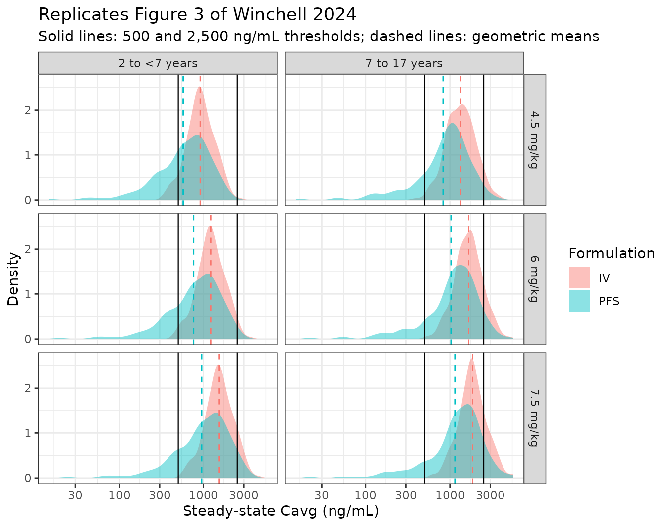
cavg_subject |>
  group_by(agegrp, dose_label, form) |>
  summarise(`% >=500 ng/mL` = 100 * mean(PPORRES >= 500),
            `% 500 to <2500` = 100 * mean(PPORRES >= 500 & PPORRES < 2500),
            .groups = "drop") |>
  rename("Age group" = agegrp, "Dose" = dose_label, "Formulation" = form) |>
  knitr::kable(digits = 1,
caption = "Attainment of the Winchell 2024 PK target (Cavg >= 500 ng/mL).")| Age group | Dose | Formulation | % >=500 ng/mL | % 500 to <2500 |
|---|---|---|---|---|
| 2 to <7 years | 4.5 mg/kg | IV | 93.5 | 93.0 |
| 2 to <7 years | 4.5 mg/kg | PFS | 67.0 | 67.0 |
| 2 to <7 years | 6 mg/kg | IV | 99.0 | 96.5 |
| 2 to <7 years | 6 mg/kg | PFS | 76.0 | 75.0 |
| 2 to <7 years | 7.5 mg/kg | IV | 100.0 | 90.0 |
| 2 to <7 years | 7.5 mg/kg | PFS | 82.0 | 77.0 |
| 7 to 17 years | 4.5 mg/kg | IV | 99.5 | 93.5 |
| 7 to 17 years | 4.5 mg/kg | PFS | 82.0 | 79.5 |
| 7 to 17 years | 6 mg/kg | IV | 100.0 | 87.0 |
| 7 to 17 years | 6 mg/kg | PFS | 87.0 | 80.0 |
| 7 to 17 years | 7.5 mg/kg | IV | 100.0 | 80.5 |
| 7 to 17 years | 7.5 mg/kg | PFS | 87.5 | 78.5 |
The paper’s headline conclusion – that the 6 mg/kg per day regimen puts more than 90% of pediatric patients in both age strata above the 500 ng/mL Cavg target, by either route – is reproduced.
Concentration-time profile over the IV to PFS switch
The clinical regimen starts IV and optionally switches to oral PFS between days 10 and 18. A typical-value profile over the switch illustrates the structural model; it is not a published figure.
switch_wt <- 28.6
switch_amt <- min(6 * switch_wt, 300)
switch_events <- bind_rows(
  # IV BID on day 1, IV QD days 2-10, PFS QD days 10-14.
  data.frame(time = c(0, 12), amt = switch_amt, cmt = "central", evid = 1L),
  data.frame(time = 24 * (1:9), amt = switch_amt, cmt = "central", evid = 1L),
  data.frame(time = 24 * (10:14), amt = switch_amt, cmt = "depot", evid = 1L),
  data.frame(time = seq(0, 24 * 15, by = 0.25), amt = 0, cmt = "central", evid = 0L)
) |>
  mutate(id = 1L, WT = switch_wt, ii = 0, ss = 0L) |>
  arrange(time, -evid)

switch_sim <- rxode2::rxSolve(mod, switch_events, omega = NA,
                              returnType = "data.frame") |>
  filter(!is.na(Cc))

ggplot(switch_sim, aes(time / 24, Cc)) +
  geom_line() +
  geom_vline(xintercept = 10, linetype = "dashed") +
  geom_hline(yintercept = 500, colour = "grey40") +
  labs(x = "Time (days)", y = "Posaconazole concentration (ng/mL)",
       title = "Typical-value profile, 6 mg/kg QD in a 28.6 kg patient",
       subtitle = "Dashed line: switch from IV solution to oral PFS on day 10") +
  theme_bw()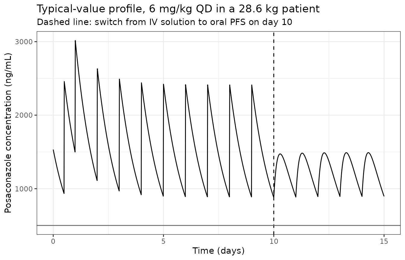
Assumptions and deviations
-
Allometric reference weight (28.6 kg) is not stated by the
paper. Winchell 2024 reports estimated allometric exponents on
CL and Vc but never prints the body-weight normalisation constant used
in the NONMEM covariate model, and neither does the supplement. 28.6 kg
– the overall median weight of the analysis population (Table 1, “All (N
= 114)”) – was adopted. It is supported three ways: (i) back-solving the
Supplementary Table 2 IV Cavg geometric means brackets the reference at
roughly 29-35 kg and the weight-band fit to Supplementary Table 3 gives
~35 kg; (ii) the conventional 70 kg is refuted decisively,
overpredicting the Supplementary Table 2 IV Cavg values by 54-78%;
- the same authors’ adult posaconazole tablet model, which this
analysis was based on, normalises body weight to its own
simulation-cohort median (
vanIersel_2018_posaconazole). A value in the low 30s would fit the supplement’s tables marginally better, but is printed nowhere in the paper; choosing it would be fitting the model to a validation target rather than transcribing the source, so the published median was used instead. Users who need the best agreement with Supplementary Table 3 specifically can rescalelclandlvcaccordingly.
- the same authors’ adult posaconazole tablet model, which this
analysis was based on, normalises body weight to its own
simulation-cohort median (
-
The CL-Vc random-effect correlation is reported to exist but
not quantified. Results “Final model” lists “correlation
between CL and Vc” among the final model’s features, but no correlation
coefficient or covariance appears in Table 2, in the text, or in the
supplement. The
ini()block keeps the two-eta block structure with the off-diagonal set to 0 rather than inventing a covariance. Simulated marginal distributions of CL and Vc are unaffected; only their joint dependence is. - The bioavailability random effect is encoded at its reported magnitude (logit-domain SD 2.02), which is larger than the paper’s own simulations behave as if they used. Footnote c’s 8%-99% interval confirms 2.02 as the reported SD exactly, so that is what the model file carries. The consequence is a systematic ~20% underprediction of the Supplementary Table 2 and Table 3 PFS results, quantified above and attributable to the 42% shrinkage the paper reports on this random effect. This was not tuned away.
- IIV magnitudes are read as log-scale SDs, per Table 2 footnote b (“a CV%, calculated by the square root of Omega, multiplied by 100”), so omega^2 = 0.371^2 and 0.277^2 directly, rather than via the lognormal omega^2 = log(1 + CV^2) conversion. Footnote c’s treatment of the F1 entry as a bare logit-domain SD is consistent with that reading of the column.
- IV doses are modelled as boluses into the central compartment. This follows Methods (“IV administration being assumed to be directed into the central compartment”); the paper does not report an infusion duration in the model, and Cavg and Cmin are insensitive to it. Cmax and Tmax after an IV dose would be, so no IV Cmax comparison is attempted here.
- The virtual cohort is reconstructed from Table 1, not from the paper’s simulation cohort, which pooled P097 with the unreported P032 weight distribution. The consequences are quantified in the cohort-diagnostic section above.
- Concentrations below the 5.00 ng/mL LLOQ were excluded from the original analysis rather than modelled with an M3-type likelihood; the packaged model carries no LLOQ handling.
-
Simulated exposures use IPRED (
Cc), without residual error. The paper’s Cavg and Cmin are model-derived exposure metrics, so residual variability is not applicable to them. - Absolute dose cap. The 300 mg cap of the source protocol and simulations is applied in the event tables, not in the model file, since it is a dosing rule rather than a model parameter.