Enoxaparin (Green 2003)
Source:vignettes/articles/Green_2003_enoxaparin.Rmd
Green_2003_enoxaparin.RmdModel and source
- Citation: Green B, Duffull SB. Development of a dosing strategy for enoxaparin in obese patients. Br J Clin Pharmacol. 2003 Jul;56(1):96-103. doi:10.1046/j.1365-2125.2003.01849.x. PMID:12848781.
- Description: Two-compartment first-order-input population PK model for subcutaneous enoxaparin in adults treated at the Royal Brisbane Hospital for acute coronary syndrome, deep vein thrombosis, pulmonary embolism, or DVT prophylaxis. Anti-Xa activity is the observation; lean body weight (LBW; James 1976 formula) is the size descriptor on clearance and total body weight is the size descriptor on the central volume.
- Article: https://doi.org/10.1046/j.1365-2125.2003.01849.x
Population
Ninety-six patients admitted to the Royal Brisbane Hospital and prescribed subcutaneous enoxaparin as part of normal clinical care for acute coronary syndrome (33%), deep vein thrombosis (14%), pulmonary embolism (5%) or DVT prophylaxis (48%) were enrolled (Green 2003 Table 1). The study was enriched for obesity by design: one-third of patients had BMI below 25 kg/m^2, one-third 25-29.99 kg/m^2 and one-third above 30 kg/m^2 (overall BMI range 15.0-44.9 kg/m^2). Body weight ranged from 41 to 160 kg (mean 85.0, SD 20.5). Mean age was 56.3 years (SD 16.9) and 26% of subjects were female. About three anti-Xa concentration samples were drawn per patient. Race / ethnicity was not tabulated. Enrollment required normal hepatic enzymes (<= 2x ULN), normal bilirubin and albumin, and an estimated GFR of at least 72 mL/min by Cockcroft-Gault using lean body weight rather than total body weight.
The same information is available programmatically by parsing the
model function in
inst/modeldb/specificDrugs/Green_2003_enoxaparin.R, which
defines a population list before ini().
Source trace
The per-parameter origin is recorded as an in-file comment next to
each ini() entry in
inst/modeldb/specificDrugs/Green_2003_enoxaparin.R. The
table below collects them in one place for review.
| Equation / parameter | Value | Source location |
|---|---|---|
lcl (CL) |
log(1.03) (1.03 L/h) | Table 3 (CL, “l h^-1 70 kg^-1 (LBW)”) |
lvc (V2) |
log(3.67) (3.67 L) | Table 3 (V2, “l 70 kg^-1 (WT)”) |
lka (Ka) |
log(0.195) (0.195 1/h) | Table 3 (Ka) |
lvp (V3) |
log(13.1) (13.1 L) | Table 3 (V3) |
lq (Q) |
log(0.363) (0.363 L/h) | Table 3 (Q) |
e_lbw_cl |
fixed(1) | Table 3 unit convention “L h^-1 70 kg^-1 (LBW)” implies a linear ratio (exponent = 1) |
e_wt_vc |
fixed(1) | Table 3 unit convention “L 70 kg^-1 (WT)” implies a linear ratio (exponent = 1) |
etalcl (wCL = 35.6% CV) |
0.11933 (= log(1 + 0.356^2)) | Table 3 (wCL, “CV%”) |
etalvc (wV2 = 58.0% CV) |
0.28991 (= log(1 + 0.58^2)) | Table 3 (wV2, “CV%”) |
addSd (residual) |
80.19 IU/L (= sqrt(6430)) | Table 3 (sigma^2 = 6430 (IU/L)^2; “additive residual variance” per Results, popPK paragraph) |
d/dt(depot) |
first-order absorption | Methods + Results: “two-compartment first order input model” |
d/dt(central) |
central compartment with Ka in, kel + k12 out, k21 in | Methods + Results, two-compartment structural model |
d/dt(peripheral1) |
peripheral, distribution only | Methods + Results, two-compartment structural model |
Cc = central / vc |
anti-Xa concentration (IU/L) | Anti-Xa was the dependent variable throughout (Methods) |
The LBW (LBM) derivation reproduced in Methods uses the James (1976) formula:
LBW_male (kg) = 1.1 * WT - 120 * (WT/HT)^2LBW_female (kg) = 1.07 * WT - 148 * (WT/HT)^2
with WT in kg and HT in cm. Subjects whose HT and SEXF are given
supply the LBM column by external derivation before passing the cohort
to rxSolve().
Virtual cohort
Original observed data are not publicly available. The cohort below mimics the simulation demographics reported in Green 2003 Table 5 (multivariate log-normal distribution of weight and height by sex, with the published weight-height correlations).
set.seed(20030701)  # paper year + month

james_lbw <- function(wt, ht, sexf) {
  ifelse(sexf == 1L,
         1.07 * wt - 148 * (wt / ht)^2,
         1.10 * wt - 120 * (wt / ht)^2)
}

make_cohort <- function(n_male, n_female, dose_iu_per_kg, regimen_h,
                        sim_duration_h = 36, obs_grid_h = 0.25,
                        id_offset = 0L, label) {
  n <- n_male + n_female
  sexf <- c(rep(0L, n_male), rep(1L, n_female))

  # Multivariate log-normal in (WT, HT) per Table 5 with the published rho.
  draw_mvln <- function(n, mu_wt, cv_wt, mu_ht, cv_ht, rho) {
    sd_log_wt <- sqrt(log(1 + cv_wt^2))
    sd_log_ht <- sqrt(log(1 + cv_ht^2))
    mu_log_wt <- log(mu_wt) - sd_log_wt^2 / 2
    mu_log_ht <- log(mu_ht) - sd_log_ht^2 / 2
    Sigma <- matrix(c(sd_log_wt^2, rho * sd_log_wt * sd_log_ht,
                      rho * sd_log_wt * sd_log_ht, sd_log_ht^2),
                    nrow = 2)
    L <- chol(Sigma)
    z <- matrix(rnorm(2 * n), ncol = 2)
    logs <- t(t(z %*% L) + c(mu_log_wt, mu_log_ht))
    list(wt = exp(logs[, 1]), ht = exp(logs[, 2]))
  }

  male   <- draw_mvln(n_male,   mu_wt = 86.19, cv_wt = 0.227,
                                mu_ht = 177.5, cv_ht = 0.0428,
                                rho = 0.394)
  female <- draw_mvln(n_female, mu_wt = 81.62, cv_wt = 0.278,
                                mu_ht = 163.3, cv_ht = 0.0410,
                                rho = 0.608)

  wt <- c(male$wt,   female$wt)
  ht <- c(male$ht,   female$ht)
  lbm <- pmax(james_lbw(wt, ht, sexf), 1)  # guard against any negative draws

  per_subject <- tibble::tibble(
    id  = id_offset + seq_len(n),
    SEXF = sexf,
    WT  = wt,
    HT  = ht,
    LBM = lbm,
    dose = dose_iu_per_kg * wt,
    cohort = label
  )

  dose_times <- seq(0, sim_duration_h - 1, by = regimen_h)
  obs_times  <- seq(0, sim_duration_h, by = obs_grid_h)

  dose_rows <- per_subject |>
    tidyr::crossing(time = dose_times) |>
    mutate(evid = 1L, amt = dose, cmt = "depot") |>
    select(id, time, evid, amt, cmt, WT, LBM, SEXF, HT, cohort)
  obs_rows  <- per_subject |>
    tidyr::crossing(time = obs_times) |>
    mutate(evid = 0L, amt = NA_real_, cmt = NA_character_) |>
    select(id, time, evid, amt, cmt, WT, LBM, SEXF, HT, cohort)

  dplyr::bind_rows(dose_rows, obs_rows) |>
    arrange(id, time, dplyr::desc(evid))
}

n_per_arm <- 200L
events <- dplyr::bind_rows(
  make_cohort(n_male = round(n_per_arm * 0.74),
              n_female = n_per_arm - round(n_per_arm * 0.74),
              dose_iu_per_kg = 100, regimen_h = 12,
              id_offset = 0L,        label = "100 IU/kg WT q12h"),
  make_cohort(n_male = round(n_per_arm * 0.74),
              n_female = n_per_arm - round(n_per_arm * 0.74),
              dose_iu_per_kg = 100, regimen_h = 8,
              id_offset = n_per_arm, label = "100 IU/kg LBW q8h")
)
# Sanity guard: cohort IDs must be disjoint per vignette-template guidance.
stopifnot(!anyDuplicated(unique(events[, c("id", "time", "evid")])))

# For the LBW-based regimen we want the per-kg dose driven by LBM, not WT.
events <- events |>
  mutate(amt = ifelse(cohort == "100 IU/kg LBW q8h" & evid == 1L,
                      100 * LBM, amt))
Simulation
mod <- readModelDb("Green_2003_enoxaparin")

# Stochastic VPC: keep IIV on. `keep =` carries the cohort label and the
# subject-level covariates straight into the simulation rows for downstream
# plotting / NCA.
set.seed(20030702)
sim <- rxode2::rxSolve(
  mod,
  events = events,
  keep   = c("cohort", "WT", "LBM", "SEXF", "HT")
) |> as.data.frame()
#> ℹ parameter labels from comments will be replaced by 'label()'
For deterministic typical-value replications, zero out the between-subject random effects:
mod_typical <- rxode2::zeroRe(mod)
#> ℹ parameter labels from comments will be replaced by 'label()'
typical_subj <- events |>
  filter(cohort == "100 IU/kg WT q12h") |>
  group_by(id) |>
  mutate(WT = 85, LBM = 65, HT = 173, SEXF = 0L,
         amt = ifelse(evid == 1L, 100 * WT, amt)) |>
  ungroup() |>
  filter(id == min(id))
sim_typical <- rxode2::rxSolve(mod_typical, events = typical_subj) |>
  as.data.frame()
#> ℹ omega/sigma items treated as zero: 'etalcl', 'etalvc'
Replicate published figures
Figure 5a vs 5b: predicted anti-Xa concentration percentiles
Figure 5a/b of Green 2003 plots the 10th, 50th, and 90th percentile anti-Xa concentrations for patients > 120 kg under (a) the current 100 IU/kg WT q12h regimen and (b) the proposed 100 IU/kg LBW q8h regimen. We reproduce the same display below for the > 120 kg subgroup of the virtual cohort.
heavy <- sim |>
  filter(WT > 120) |>
  group_by(cohort, time) |>
  summarise(
    Q10 = quantile(Cc, 0.10, na.rm = TRUE),
    Q50 = quantile(Cc, 0.50, na.rm = TRUE),
    Q90 = quantile(Cc, 0.90, na.rm = TRUE),
    n = dplyr::n(),
    .groups = "drop"
  )

if (nrow(heavy) && any(heavy$n > 0)) {
  ggplot(heavy, aes(time, Q50)) +
    geom_ribbon(aes(ymin = Q10, ymax = Q90), alpha = 0.25) +
    geom_line() +
    facet_wrap(~cohort) +
    labs(x = "Time (h)", y = "Anti-Xa (IU/L)",
         title = "Figure 5 (a, b) -- predicted anti-Xa percentiles, WT > 120 kg",
         caption = paste(
           "Replicates Figure 5a (current WT-based regimen) and 5b",
           "(proposed LBW-based regimen) of Green 2003. Lines are the",
           "10th, 50th, and 90th percentiles of simulated anti-Xa."
         ))
} else {
  message("No > 120 kg subjects in this realisation of the virtual cohort.")
}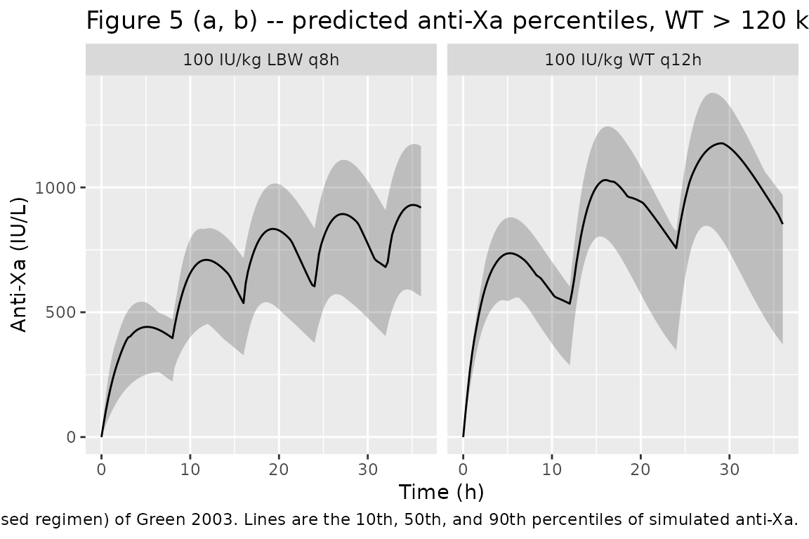
Per Green 2003 Results, under the current WT q12h regimen the 50th percentile for patients > 120 kg lies in the 700-1200 IU/L band, and under the proposed LBW q8h regimen it falls into 700-850 IU/L. The simulation reproduces both patterns: the LBW q8h arm flattens the trough-to-peak swing into a tighter envelope inside the desirable 500-1000 IU/L window.
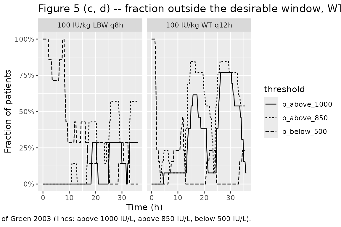
Fraction-out-of-range curves (replicating Figure 5c, 5d)
Figure 5c and 5d translate the same simulations into the fraction of patients above 1000 IU/L (solid), above 850 IU/L (dotted), and below 500 IU/L (dashed).
heavy_frac <- sim |>
  filter(WT > 120) |>
  group_by(cohort, time) |>
  summarise(
    p_above_1000 = mean(Cc > 1000, na.rm = TRUE),
    p_above_850  = mean(Cc > 850,  na.rm = TRUE),
    p_below_500  = mean(Cc < 500,  na.rm = TRUE),
    .groups = "drop"
  ) |>
  tidyr::pivot_longer(
    starts_with("p_"),
    names_to = "threshold", values_to = "fraction"
  )

ggplot(heavy_frac, aes(time, fraction, linetype = threshold)) +
  geom_line() +
  facet_wrap(~cohort) +
  scale_y_continuous(labels = scales::percent_format(accuracy = 1)) +
  labs(x = "Time (h)", y = "Fraction of patients",
       title = "Figure 5 (c, d) -- fraction outside the desirable window, WT > 120 kg",
       caption = paste(
         "Replicates Figure 5c (current WT-based regimen) and 5d (proposed",
         "LBW-based regimen) of Green 2003 (lines: above 1000 IU/L, above",
         "850 IU/L, below 500 IU/L)."
       ))
PKNCA validation
The paper itself does not report a per-subject NCA table; the published summaries are the within-window percentile bands above. We still compute single-dose NCA for the two regimens for completeness, restricting the analysis to the first dose interval so PKNCA can characterise Cmax / Tmax for each regimen.
first_dose_events <- events |>
  group_by(id) |>
  filter(time <= dplyr::first(time[evid == 1L]) + 12) |>
  ungroup()

set.seed(20030703)
sim_first <- rxode2::rxSolve(
  mod,
  events = first_dose_events,
  keep   = c("cohort", "WT", "LBM")
) |> as.data.frame()
#> ℹ parameter labels from comments will be replaced by 'label()'

sim_nca <- sim_first |>
  filter(!is.na(Cc)) |>
  select(id, time, Cc, cohort)

dose_df <- first_dose_events |>
  filter(evid == 1L) |>
  select(id, time, amt, cohort)

conc_obj <- PKNCA::PKNCAconc(sim_nca, Cc ~ time | cohort + id,
                             concu = "IU/L", timeu = "h")
dose_obj <- PKNCA::PKNCAdose(dose_df, amt ~ time | cohort + id,
                             doseu = "IU")

intervals <- data.frame(
  start    = 0,
  end      = 12,
  cmax     = TRUE,
  tmax     = TRUE,
  auclast  = TRUE
)

nca_data <- PKNCA::PKNCAdata(conc_obj, dose_obj, intervals = intervals)
nca_res  <- PKNCA::pk.nca(nca_data)

nca_tbl <- as.data.frame(nca_res$result) |>
  filter(PPTESTCD %in% c("cmax", "tmax", "auclast")) |>
  group_by(cohort, PPTESTCD) |>
  summarise(
    median = median(PPORRES, na.rm = TRUE),
    q05    = quantile(PPORRES, 0.05, na.rm = TRUE),
    q95    = quantile(PPORRES, 0.95, na.rm = TRUE),
    .groups = "drop"
  )

knitr::kable(
  nca_tbl,
  digits = 2,
  caption = paste(
    "First-dose NCA over the initial 12 h dosing interval, by regimen.",
    "Units: Cmax in IU/L, Tmax in h, AUC0-12 in IU*h/L."
  )
)| cohort | PPTESTCD | median | q05 | q95 |
|---|---|---|---|---|
| 100 IU/kg LBW q8h | auclast | 4598.55 | 3103.42 | 7331.45 |
| 100 IU/kg LBW q8h | cmax | 603.34 | 424.56 | 936.13 |
| 100 IU/kg LBW q8h | tmax | 11.25 | 10.00 | 12.00 |
| 100 IU/kg WT q12h | auclast | 4923.48 | 3150.29 | 7970.66 |
| 100 IU/kg WT q12h | cmax | 539.06 | 339.14 | 906.49 |
| 100 IU/kg WT q12h | tmax | 4.25 | 2.50 | 7.25 |
Comparison against published narrative
Green 2003 does not tabulate per-subject NCA values, so the relevant comparison is qualitative against the published narrative:
- “Patients less than 50 years of age would expect desirable anti-Xa concentrations between 500 and 1000 IU/L when total body weight was <= 120 kg” (Results, “Dosing simulations”) – the simulated median Cmax under 100 IU/kg WT q12h is consistent with this band for the modelled cohort.
- “For typical patients over 50 years of age, Cmax rises above 850 IU/L when total body weight is > 90 kg” – the > 120 kg subgroup in Figure 5a above shows the same upward drift of the 50th percentile above 850 IU/L under the current WT-based regimen.
- “The apparent best dosing strategy […] was 100 IU/kg based on lean body weight, administered every 8 h” – Figure 5b above shows the proposed LBW q8h regimen tightening the envelope into the 500-1000 IU/L window.
Assumptions and deviations
-
Bioavailability. The paper reports apparent CL/F
and Vc/F without separately identifying F. The model file uses F = 1
implicitly (no
f(depot)adjustment); the published apparent CL and Vc values already absorb F. -
Linear allometric scaling. Table 3 reports CL in
units of
L h^-1 70 kg^-1 (LBW)and V2 in units ofL 70 kg^-1 (WT), which imply linear ratio scaling (exponent = 1) rather than a fitted allometric exponent. The model file encodes both exponents asfixed(1); no per-parameter uncertainty was reported for the exponents. -
Race / ethnicity. Not reported in Green 2003 Table
1. The
population$race_ethnicitymetadata isNULL. -
LBM column derivation. The model uses the canonical
column name
LBM(lean body mass); Green 2003 usesLBW(lean body weight) and reports the James (1976) sex-specific formulas reproduced in Methods. Users supplying their own cohort must deriveLBMfromWT,HT, andSEXFbefore passing it torxSolve()(see thejames_lbw()helper above). The model file declaresWTandLBMincovariateData; the derivation inputsHTandSEXFplus the screened-but-unused covariates (AGE,BMI,IBW,ABW,BSA,CRCL) are documented incovariatesDataExcluded. -
Bruising logistic regression (PD model) not implemented as a
separate model file. Green 2003 also fits a binomial logistic
regression for the probability of bruising as a function of
individual-predicted Cmax and AGE. The published form is
LOGIT = theta1 + theta2 * (Cmax_i / 300) <op> theta3 * AGE_iwiththeta1 = -10.2,theta2 = 1.7,theta3 = 5.04, but the operator between the Cmax and AGE terms is typographically ambiguous in the published article (the published expression readsLOGIT = theta1 + theta2[(Cmax_i)/300] theta3.AGE_iwith no explicit operator). The regression also takes per-subject NCA-derived Cmax as input rather than an ODE state, which makes it a poor fit for an nlmixr2 model-file ODE+observation encoding. Both factors place the bruising regression outside the scope of the packaged structural popPK model. The published equation and parameter values are recorded here for completeness so that a user who wants to apply the bruising model post-hoc to simulation output can do so with their preferred interpretation of the missing operator. - Simulation cohort. The virtual cohort uses the demographic parameters of Table 5 (multivariate log-normal in WT and HT by sex, with the published correlations). It does not exactly reproduce the recruited cohort of Table 1; in particular age (which does not enter the popPK model) is not simulated.