Isoniazid (Vinnard 2017)

Model and source

#> Warning: some etas defaulted to non-mu referenced, possible parsing error: etaiov_cl_1, etaiov_cl_2
#> as a work-around try putting the mu-referenced expression on a simple line

• Citation: Vinnard C, Ravimohan S, Tamuhla N, Ivaturi V, Pasipanodya J, Srivastava S, Modongo C, Zetola NM, Weissman D, Gumbo T, Bisson GP. (2017). Isoniazid clearance is impaired among human immunodeficiency virus/tuberculosis patients with high levels of immune activation. Br J Clin Pharmacol 83(4):801-811. doi:10.1111/bcp.13172.

• Description: Two-compartment population PK model with first-order absorption and an absorption lag time for oral isoniazid in HIV/tuberculosis co-infected adults in Botswana (Vinnard 2017). NAT2 acetylator genotype (slow acetylator as the reference, with proportional shifts for the intermediate and rapid phenotypes) and systemic immune activation (percent CD38 and HLA-DR co-expression on CD8+ T cells, entered as a median-normalised power term) act on apparent oral clearance; between-subject variability on CL/F, V/F and the absorption lag time, and inter-occasion variability on CL/F across the pre-ART and post-ART pharmacokinetic visits.

• Article: Br J Clin Pharmacol 2017;83(4):801-811

• PubMed Central: PMC5346858

Vinnard and colleagues asked whether systemic immune activation, the hallmark of both untreated HIV infection and active tuberculosis, impairs isoniazid clearance over and above the well-established effect of NAT2 acetylator genotype. Forty ART-naive HIV/TB patients in Gaborone, Botswana were sampled intensively before starting antiretroviral therapy, and 24 of them again about a month after. The answer was yes: after accounting for NAT2 genotype, a higher percentage of circulating CD8+ T cells co-expressing CD38 and HLA-DR predicted lower isoniazid clearance, and therefore higher isoniazid exposure.

Population

Sixty-one HIV/TB patients were screened and 40 enrolled (Table 1, journal page 805): 45% women, median age 32 years (IQR 27-43), median weight 55.0 kg (IQR 49.3-59.3), median creatinine clearance 102.1 mL/min (IQR 92.5-114.1). All were citizens of Botswana, ART-naive at enrolment, newly diagnosed with pulmonary TB, and established on a standard WHO first-line regimen dosed by weight band. Creatinine clearance below 50 mL/min and transaminases above three times the upper limit of normal were exclusion criteria.

The first pharmacokinetic visit occurred 5 to 28 days after starting anti-TB therapy (median 20 days), before any ART. Twenty-four patients returned for a second visit after a median of 33 days of tenofovir/emtricitabine/efavirenz. Between visits the median CD4+ count rose from 238 to 308 cells/uL and HIV viral load fell in all but one participant, while the immune-activation marker %CD38+DR+CD8+ fell from a median of 36.9% (IQR 27.7-45.7) to 24.8% (IQR 21.9-35.9) – though individual trajectories went both ways.

NAT2 genotype was resolved in 38 of 40 participants: 7 slow (18%), 18 intermediate (45%) and 13 rapid (33%) acetylators, with 2 ambiguous.

Serum isoniazid was measured at 0, 0.3, 0.9, 2.2, 4.5 and 8 h post-dose by stable-isotope dilution LC-ESI-MS/MS (LLOQ 0.16 mg/L). Estimation used FOCE in Phoenix NLME 1.3.

The same information is available programmatically:

str(rxode2::rxode(readModelDb("Vinnard_2017_isoniazid"))$population)
#> Warning: some etas defaulted to non-mu referenced, possible parsing error: etaiov_cl_1, etaiov_cl_2
#> as a work-around try putting the mu-referenced expression on a simple line
#> List of 16
#>  $ species         : chr "human"
#>  $ n_subjects      : int 40
#>  $ n_studies       : int 1
#>  $ age_range       : chr "21 years and older (enrolment criterion)"
#>  $ age_median      : chr "32 years (IQR 27-43) at visit 1; 32 years (IQR 28-43) at visit 2"
#>  $ weight_range    : chr "Not tabulated as a range; median 55.0 kg (IQR 49.3-59.3) at visit 1 and 56.6 kg (IQR 52.5-61.8) at visit 2"
#>  $ weight_median   : chr "55.0 kg"
#>  $ sex_female_pct  : num 45
#>  $ race_ethnicity  : chr "Citizens of Botswana (sub-Saharan African); detailed ancestry not reported."
#>  $ disease_state   : chr "ART-naive HIV-infected adults newly diagnosed with pulmonary TB and established on a standard WHO first-line an"| __truncated__
#>  $ dose_range      : chr "Oral isoniazid once daily as part of a first-line fixed-dose combination, dosed by WHO weight band (Methods 'St"| __truncated__
#>  $ regions         : chr "Botswana (Gaborone; 22 public clinics and Princess Marina Hospital)."
#>  $ renal_function  : chr "Creatinine clearance below 50 mL/min was an exclusion criterion; median CrCl 102.1 mL/min (IQR 92.5-114.1) at visit 1."
#>  $ hepatic_function: chr "Alanine or aspartate transaminase above 3 times the upper limit of normal was an exclusion criterion."
#>  $ co_medication   : chr "First-line antitubercular fixed-dose combination therapy at both visits; tenofovir/emtricitabine/efavirenz ART "| __truncated__
#>  $ notes           : chr "Prospective observational two-visit design. 61 patients were screened and 40 enrolled and sampled at visit 1 (m"| __truncated__

Source trace

Every ini() entry carries an in-file comment naming its source location in inst/modeldb/specificDrugs/Vinnard_2017_isoniazid.R. They are collected here for review.

Equation / parameter	Value	Source location
lka	log(0.88)	Table 2, journal page 808: Ka = 0.88 1/h (RSE 12.45%)
lcl	log(10.99)	Table 2: CL = 10.99 L/h (RSE 9.86%)
lvc	log(5.55)	Table 2: V = 5.55 L (RSE 48.11%)
lvp	log(17.54)	Table 2: V2 = 17.54 L (RSE 16.29%)
lq	log(11.61)	Table 2: Q = 11.61 L/h (RSE 34.06%)
ltlag	log(0.25)	Table 2: Tlag = 0.25 h (RSE 11.67%)
e_nat2_int_cl	0.63	Table 2: Theta(Intermediate NAT2) = 0.63 (RSE 30.62%), 95% CI 0.30 to 1.06
e_nat2_rapid_cl	1.65	Table 2: Theta(Rapid NAT2) = 1.65 (RSE 18.22%), 95% CI 1.14 to 2.25
e_cd8_cd38dr_pct_cl	-0.31	Table 2: Theta(%CD38 + HLA-DR + |CD8) = -0.31 (RSE 40.06%), 95% CI -0.57 to -0.07
etalcl	0.08237	Table 2: BSV-CL 29.3% CV; omega^2 = log(1 + 0.293^2)
etalvc	1.07858	Table 2: BSV-V 139.3% CV; omega^2 = log(1 + 1.393^2)
etaltlag	0.00937	Table 2: BSV-Tlag 9.7% CV; omega^2 = log(1 + 0.097^2)
etaiov_cl_1, etaiov_cl_2	0.00202	Table 2: BSV-IOV 4.5% CV; omega^2 = log(1 + 0.045^2); one variance shared across both occasions
addSd	0.06	Table 2: additive error SD = 0.06 mg/L (RSE 16.68%)
propSd	0.25	Table 2: proportional error = 0.25 (RSE 12.27%)
Two-compartment ODEs, first-order absorption	n/a	Results paragraph 3: “best described by a two-compartment model with first-order elimination”
alag(depot) <- tlag	n/a	Results paragraph 3: “Fit of the concentrations during the absorptive phase was improved with the use of a time-lag absorption model”
BSV on CL, V, Tlag only	n/a	Results paragraph 4: “BSV on CL, V, and Tlag (Table 2)”; eta shrinkage 10.0% / 12.8% / 43.0%
IOV on CL across two visits	n/a	Results paragraph 4: “we introduced interoccasional variability (IOV) on CL into the population PK model”
Combined additive + proportional error	n/a	Results paragraph 3: “a combined additive/proportional residual error model”
Normalisation of %CD38+DR+CD8+ at 36.9%	n/a	Table 1, journal page 805: visit-1 cohort median 36.9% (IQR 27.7-45.7, n = 38)
NAT2_SLOW as covariate-model reference	n/a	Table 2 prints thetas for the intermediate and rapid levels only, so slow is the omitted reference
Covariate functional forms	n/a	Not printed by the paper. Recovered from published anchors; see the next section
Dose 300 mg for the simulations below	n/a	Not tabulated by the paper. Implied by the Figure 3 CL/AUC pairs; see Assumptions

Recovering the covariate functional forms

The paper gives point estimates for three covariate coefficients but never writes the covariate equation. Phoenix NLME admits several standard forms, and they are not interchangeable: for the rapid-acetylator coefficient of 1.65 a proportional (1 + theta) form means a 2.65-fold clearance increase while an exponential exp(theta) form means a 5.21-fold increase. Four independent anchors published in the paper settle it.

theta_int   <-  0.63
theta_rapid <-  1.65
theta_cd38  <- -0.31
cl_ref      <- 10.99   # Table 2 typical value = the slow-acetylator reference
cd38_ref    <- 36.9    # Table 1 visit-1 median, the normalising value

# The two candidate categorical forms.
cl_prop <- cl_ref * c(slow = 1,
                      intermediate = 1 + theta_int,
                      rapid        = 1 + theta_rapid)
cl_expo <- cl_ref * c(slow = 1,
                      intermediate = exp(theta_int),
                      rapid        = exp(theta_rapid))

# --- Anchor 1: Figure 3A (journal page 809) plots every individual's predicted
# CL/F, faceted by NAT2 genotype, pre-ART vs post-ART. These are the pre-ART
# per-genotype medians read off that panel by on-screen digitisation
# (approximately +/- 10%; the panel's y-axis tops out just above 36 L/h).
fig3a_median_cl <- c(slow = 10.2, intermediate = 19.0, rapid = 26.5)

anchor1 <- tibble::tibble(
  genotype       = names(fig3a_median_cl),
  `Figure 3A median CL/F (L/h)` = as.numeric(fig3a_median_cl),
  `Proportional form (L/h)`     = as.numeric(cl_prop),
  `Exponential form (L/h)`      = as.numeric(cl_expo),
  `Proportional % diff`         = 100 * (cl_prop - fig3a_median_cl) / fig3a_median_cl,
  `Exponential % diff`          = 100 * (cl_expo - fig3a_median_cl) / fig3a_median_cl
)
knitr::kable(
  anchor1, digits = 1,
  caption = paste(
    "Anchor 1. Per-genotype typical CL/F under each candidate form, against the",
    "digitised pre-ART medians of Figure 3A. The exponential form puts the rapid",
    "typical value at 57 L/h, off the published panel's axis entirely."
  )
)

Anchor 1. Per-genotype typical CL/F under each candidate form, against the digitised pre-ART medians of Figure 3A. The exponential form puts the rapid typical value at 57 L/h, off the published panel’s axis entirely.

genotype	Figure 3A median CL/F (L/h)	Proportional form (L/h)	Exponential form (L/h)	Proportional % diff	Exponential % diff
slow	10.2	11.0	11.0	7.7	7.7
intermediate	19.0	17.9	20.6	-5.7	8.6
rapid	26.5	29.1	57.2	9.9	115.9

# --- Anchor 2: Figure 2A (journal page 808) box-plots eta_CL from the BASE
# model (no covariates) by genotype. Digitised medians:
fig2a_eta_median <- c(slow = -0.53, intermediate = 0.07, rapid = 0.40)

# A base model's etas centre on the population geometric mean, so each form
# predicts eta_g = log(factor_g) - E[log(factor)] over the published genotype
# frequencies (7 slow / 18 intermediate / 13 rapid of 38 non-ambiguous).
geno_freq <- c(slow = 7, intermediate = 18, rapid = 13)
geno_freq <- geno_freq / sum(geno_freq)

centred_eta <- function(cl_vec) {
  lf <- log(cl_vec / cl_ref)
  lf - sum(geno_freq * lf)
}

anchor2 <- tibble::tibble(
  genotype                  = names(fig2a_eta_median),
  `Figure 2A median eta_CL` = as.numeric(fig2a_eta_median),
  `Proportional form`       = as.numeric(centred_eta(cl_prop)),
  `Exponential form`        = as.numeric(centred_eta(cl_expo))
)
rmse <- function(a, b) sqrt(mean((a - b)^2))
rmse_prop <- rmse(anchor2$`Figure 2A median eta_CL`, anchor2$`Proportional form`)
rmse_expo <- rmse(anchor2$`Figure 2A median eta_CL`, anchor2$`Exponential form`)

knitr::kable(
  anchor2, digits = 3,
  caption = sprintf(
    paste("Anchor 2. Base-model eta_CL by genotype (Figure 2A) against each form's",
          "frequency-centred prediction. RMSE: proportional %.3f, exponential %.3f."),
    rmse_prop, rmse_expo
  )
)

Anchor 2. Base-model eta_CL by genotype (Figure 2A) against each form’s frequency-centred prediction. RMSE: proportional 0.087, exponential 0.343.

genotype	Figure 2A median eta_CL	Proportional form	Exponential form
slow	-0.53	-0.565	-0.863
intermediate	0.07	-0.076	-0.233
rapid	0.40	0.410	0.787

# --- Anchor 3: the paper reports the BSV-CL sequence as covariates were added
# (Results paragraphs 3-4): 45.9% in the base model, 32.0% after NAT2, 29.3%
# after adding immune activation. The variance a covariate removes from
# log-CL is therefore recoverable.
cv_to_omega <- function(cv) sqrt(log(1 + cv^2))
omega_base <- cv_to_omega(0.459)
omega_nat2 <- cv_to_omega(0.320)
omega_fin  <- cv_to_omega(0.293)

sd_explained_nat2 <- sqrt(omega_base^2 - omega_nat2^2)
sd_explained_cd38 <- sqrt(omega_nat2^2 - omega_fin^2)

# What each form actually contributes, over the published genotype frequencies.
sd_of <- function(cl_vec) {
  lf <- log(cl_vec / cl_ref)
  sqrt(sum(geno_freq * lf^2) - sum(geno_freq * lf)^2)
}

# The immune-activation term contributes theta * SD(log(CD38 / ref)). Table 1's
# visit-1 IQR 27.7 to 45.7 gives SD(log CD38) = log(45.7 / 27.7) / 1.349.
sd_log_cd38 <- log(45.7 / 27.7) / (2 * qnorm(0.75))

anchor3 <- tibble::tibble(
  Covariate = c("NAT2 genotype", "NAT2 genotype", "%CD38+DR+CD8+"),
  Form      = c("proportional (1 + theta)", "exponential exp(theta)",
                "median-normalised power"),
  `SD of log-CL contributed` = c(sd_of(cl_prop), sd_of(cl_expo),
                                 abs(theta_cd38) * sd_log_cd38),
  `SD required by published BSV drop` = c(sd_explained_nat2, sd_explained_nat2,
                                          sd_explained_cd38)
) |>
  dplyr::mutate(Ratio = `SD of log-CL contributed` / `SD required by published BSV drop`)

knitr::kable(
  anchor3, digits = 3,
  caption = paste(
    "Anchor 3. Variance accounting. A covariate form must remove as much",
    "log-CL spread as the published BSV reduction says it did. The exponential",
    "form removes roughly twice too much."
  )
)

Anchor 3. Variance accounting. A covariate form must remove as much log-CL spread as the published BSV reduction says it did. The exponential form removes roughly twice too much.

Covariate	Form	SD of log-CL contributed	SD required by published BSV drop	Ratio
NAT2 genotype	proportional (1 + theta)	0.345	0.306	1.127
NAT2 genotype	exponential exp(theta)	0.612	0.306	2.000
%CD38+DR+CD8+	median-normalised power	0.115	0.123	0.935

# --- Anchor 4: Figure 2B (journal page 808) regresses eta_CL on
# %CD38+DR+CD8+. The plotted regression line runs from about +0.225 at x = 9.5
# to -0.29 at x = 66.5 (digitised), i.e. a slope of about -0.0090 per
# percentage point, crossing zero near the cohort median.
fig2b_slope <- (-0.29 - 0.225) / (66.5 - 9.5)

# Any covariate form normalised by a reference value has d log(CL) / dx =
# theta / ref at that reference. This is what pins the NORMALISATION: an
# un-normalised exp(theta * (x - median)) form would give a slope of -0.31 per
# percentage point, 34-fold too steep, and a fraction-scaled version would be
# about 3-fold too shallow.
slope_normalised   <- theta_cd38 / cd38_ref
slope_unnormalised <- theta_cd38
slope_fraction     <- theta_cd38 / 100

anchor4 <- tibble::tibble(
  Form = c("power / linear in x, normalised by the 36.9% median",
           "exponential, centred by subtraction, x in percent",
           "exponential, centred by subtraction, x as a fraction"),
  `d log(CL) / dx at the median` = c(slope_normalised, slope_unnormalised,
                                     slope_fraction),
  `Figure 2B regression slope`   = fig2b_slope
) |>
  dplyr::mutate(Ratio = `d log(CL) / dx at the median` / `Figure 2B regression slope`)

knitr::kable(
  anchor4, digits = 4,
  caption = paste(
    "Anchor 4. Slope of eta_CL on %CD38+DR+CD8+ (Figure 2B) against each",
    "candidate scaling. Only the median-normalised form matches."
  )
)

Anchor 4. Slope of eta_CL on %CD38+DR+CD8+ (Figure 2B) against each candidate scaling. Only the median-normalised form matches.

Form	d log(CL) / dx at the median	Figure 2B regression slope	Ratio
power / linear in x, normalised by the 36.9% median	-0.0084	-0.009	0.9298
exponential, centred by subtraction, x in percent	-0.3100	-0.009	34.3107
exponential, centred by subtraction, x as a fraction	-0.0031	-0.009	0.3431

# Gate. Each of these can go red: the exponential categorical form fails
# anchors 1 and 3 by more than 100% and 90% respectively, and the
# subtraction-centred continuous forms fail anchor 4 by 34-fold / 3-fold.
stopifnot(
  # Anchor 1: proportional form within the digitisation tolerance for all three
  # genotypes; the exponential form is not (it misses rapid by >100%).
  max(abs(anchor1$`Proportional % diff`)) < 20,
  max(abs(anchor1$`Exponential % diff`)) > 60,
  # Anchor 2: the proportional form tracks the base-model etas far better.
  rmse_prop < 0.15,
  rmse_expo > 2 * rmse_prop,
  # Anchor 3: both retained forms account for the published BSV drop within
  # 35%, and the exponential categorical alternative overshoots by >70%.
  abs(anchor3$Ratio[anchor3$Form == "proportional (1 + theta)"] - 1) < 0.35,
  abs(anchor3$Ratio[anchor3$Form == "median-normalised power"] - 1) < 0.35,
  anchor3$Ratio[anchor3$Form == "exponential exp(theta)"] > 1.7,
  # Anchor 4: median normalisation reproduces the Figure 2B slope within 20%.
  abs(slope_normalised / fig2b_slope - 1) < 0.2,
  abs(slope_unnormalised / fig2b_slope) > 20
)

All four anchors point the same way, so the packaged model implements

CL/F = 10.99 * (1 + 0.63 * I(intermediate) + 1.65 * I(rapid))
             * (%CD38+DR+CD8+ / 36.9)^(-0.31) * exp(eta_CL + kappa_IOV)

with the slow acetylator as the reference. As a fifth, external corroboration: Horita_2018_isoniazid reports CL/F of 4.44 L/h (slow) and 8.08 L/h (nonslow) in 14.3 kg Ghanaian children. Scaled allometrically to this cohort’s median 55 kg those become 12.2 and 22.2 L/h, against 10.99 L/h (slow) and a frequency-weighted 22.6 L/h (nonslow) here. The exponential form would put the nonslow value at 36 L/h.

horita_slow_55kg    <- 4.44 * (55 / 14.3)^0.75
horita_nonslow_55kg <- 8.08 * (55 / 14.3)^0.75
nonslow_w           <- geno_freq[c("intermediate", "rapid")] /
  sum(geno_freq[c("intermediate", "rapid")])
this_nonslow <- sum(nonslow_w * cl_prop[c("intermediate", "rapid")])
this_nonslow_expo <- sum(nonslow_w * cl_expo[c("intermediate", "rapid")])

tibble::tibble(
  Stratum = c("slow", "nonslow"),
  `Horita 2018 scaled to 55 kg (L/h)` = c(horita_slow_55kg, horita_nonslow_55kg),
  `This model, proportional form (L/h)` = c(cl_ref, this_nonslow),
  `This model, exponential form (L/h)`  = c(cl_ref, this_nonslow_expo)
) |>
  knitr::kable(digits = 1,
               caption = "External cross-check against the Horita 2018 isoniazid model.")

External cross-check against the Horita 2018 isoniazid model.

Stratum	Horita 2018 scaled to 55 kg (L/h)	This model, proportional form (L/h)	This model, exponential form (L/h)
slow	12.2	11.0	11
nonslow	22.2	22.6	36

stopifnot(
  abs(this_nonslow / horita_nonslow_55kg - 1) < 0.20,
  this_nonslow_expo / horita_nonslow_55kg > 1.4
)

Typical-value predictions by genotype

The paper’s own sampling design ran to 8 h, but Figure 3B reports AUC0-inf, so the checks below extend to 48 h. Isoniazid dose is 300 mg (see Assumptions).

inh_dose <- 300

mod <- readModelDb("Vinnard_2017_isoniazid")
mod_typical <- rxode2::zeroRe(mod)
#> Warning: some etas defaulted to non-mu referenced, possible parsing error: etaiov_cl_1, etaiov_cl_2
#> as a work-around try putting the mu-referenced expression on a simple line
#> Warning: some etas defaulted to non-mu referenced, possible parsing error: etaiov_cl_1, etaiov_cl_2
#> as a work-around try putting the mu-referenced expression on a simple line

genotypes <- tibble::tibble(
  genotype   = c("slow", "intermediate", "rapid"),
  NAT2_SLOW  = c(1, 0, 0),
  NAT2_RAPID = c(0, 0, 1)
)

# Dense early grid so Cmax and Tmax are resolved (Tmax is under 1 h here), then
# coarser through the terminal phase.
obs_times <- sort(unique(c(seq(0, 4, by = 0.02), seq(4, 48, by = 0.25))))

make_events <- function(row, cd38, occ, id_offset = 0L, n = 1L) {
  ev <- rxode2::et(amt = inh_dose, cmt = "depot") |>
    rxode2::et(obs_times, cmt = "central")
  ev <- as.data.frame(ev)
  out <- lapply(seq_len(n), function(i) {
    d <- ev
    d$id <- id_offset + i
    d$NAT2_SLOW  <- row$NAT2_SLOW
    d$NAT2_RAPID <- row$NAT2_RAPID
    d$CD8_CD38DR_PCT <- cd38[i]
    d$OCC <- occ
    d$genotype <- row$genotype
    d
  })
  dplyr::bind_rows(out)
}

ev_typ <- dplyr::bind_rows(lapply(seq_len(nrow(genotypes)), function(i) {
  make_events(genotypes[i, ], cd38 = cd38_ref, occ = 1L, id_offset = i - 1L)
}))

sim_typ <- rxode2::rxSolve(mod_typical, ev_typ, keep = "genotype",
                           returnType = "data.frame")
#> Warning: some etas defaulted to non-mu referenced, possible parsing error: etaiov_cl_1, etaiov_cl_2
#> as a work-around try putting the mu-referenced expression on a simple line
#> ℹ omega/sigma items treated as zero: 'etalcl', 'etalvc', 'etaltlag', 'etaiov_cl_1', 'etaiov_cl_2'
#> Warning: multi-subject simulation without without 'omega'
sim_typ <- sim_typ[!is.na(sim_typ$Cc), ]
stopifnot(nrow(sim_typ) > 0, all(sim_typ$Cc >= 0))

typ_summary <- sim_typ |>
  dplyr::group_by(genotype) |>
  dplyr::summarise(
    `CL/F (L/h)` = dplyr::first(cl),
    `V/F (L)`    = dplyr::first(vc),
    `Cmax (mg/L)` = max(Cc),
    `Tmax (h)`    = time[which.max(Cc)],
    .groups = "drop"
  ) |>
  dplyr::mutate(
    `AUC0-inf = Dose/CL (mg*h/L)` = inh_dose / `CL/F (L/h)`,
    genotype = factor(genotype, levels = genotypes$genotype)
  ) |>
  dplyr::arrange(genotype)

knitr::kable(typ_summary, digits = 2,
             caption = "Typical-value predictions at the cohort-median immune-activation level.")

Typical-value predictions at the cohort-median immune-activation level.

genotype	CL/F (L/h)	V/F (L)	Cmax (mg/L)	Tmax (h)	AUC0-inf = Dose/CL (mg*h/L)
slow	10.99	5.55	8.13	0.82	27.30
intermediate	17.91	5.55	6.52	0.70	16.75
rapid	29.12	5.55	4.98	0.60	10.30

# The typical CL/F must equal the Table 2 value times the covariate factor
# exactly -- this is deterministic, so the tolerance is numerical only.
stopifnot(all(abs(typ_summary$`CL/F (L/h)` /
                    as.numeric(cl_prop[as.character(typ_summary$genotype)]) - 1) < 1e-6))

Replicating Figure 3

Figure 3 plots each individual’s model-predicted CL/F (panel A) and AUC0-inf (panel B) by genotype. Panel A’s pre-ART medians were used as Anchor 1 above; panel B’s are compared here. Both digitised sets carry roughly +/- 10% digitisation error.

fig3_published <- tibble::tibble(
  genotype = factor(c("slow", "intermediate", "rapid"), levels = genotypes$genotype),
  cl_fig3a  = c(10.2, 19.0, 26.5),
  auc_fig3b = c(28.5, 15.2, 11.0)
)

fig3_cmp <- typ_summary |>
  dplyr::select(genotype, cl_model = `CL/F (L/h)`,
                auc_model = `AUC0-inf = Dose/CL (mg*h/L)`) |>
  dplyr::left_join(fig3_published, by = "genotype") |>
  dplyr::mutate(
    cl_pct  = 100 * (cl_model - cl_fig3a) / cl_fig3a,
    auc_pct = 100 * (auc_model - auc_fig3b) / auc_fig3b
  )

fig3_cmp |>
  dplyr::rename(
    "NAT2 genotype"                  = genotype,
    "Model CL/F (L/h)"               = cl_model,
    "Figure 3A median CL/F (L/h)"    = cl_fig3a,
    "CL % diff"                      = cl_pct,
    "Model AUC0-inf (mg*h/L)"        = auc_model,
    "Figure 3B median AUC0-inf (mg*h/L)" = auc_fig3b,
    "AUC % diff"                     = auc_pct
  ) |>
  knitr::kable(digits = 1,
               caption = "Replicates Figure 3 of Vinnard 2017 (pre-ART medians).")

Replicates Figure 3 of Vinnard 2017 (pre-ART medians).

NAT2 genotype	Model CL/F (L/h)	Model AUC0-inf (mg*h/L)	Figure 3A median CL/F (L/h)	Figure 3B median AUC0-inf (mg*h/L)	CL % diff	AUC % diff
slow	11.0	27.3	10.2	28.5	7.7	-4.2
intermediate	17.9	16.7	19.0	15.2	-5.7	10.2
rapid	29.1	10.3	26.5	11.0	9.9	-6.4

fig3_cmp |>
  dplyr::select(genotype, Model = cl_model, `Figure 3A` = cl_fig3a) |>
  tidyr::pivot_longer(-genotype, names_to = "source", values_to = "cl") |>
  ggplot(aes(genotype, cl, fill = source)) +
  geom_col(position = "dodge") +
  labs(x = "NAT2 genotype", y = "Isoniazid CL/F (L/h)",
       fill = NULL, title = "Figure 3A -- typical CL/F by NAT2 genotype",
       caption = "Replicates Figure 3A of Vinnard 2017 (pre-ART medians).")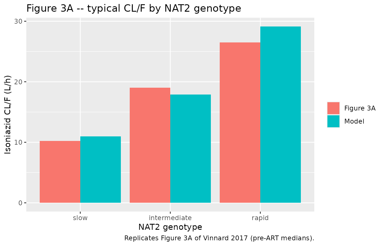

# Both panels agree within the digitisation tolerance. These are deterministic
# typical-value predictions against fixed digitised numbers, so the bound is
# not cohort-dependent.
stopifnot(
  max(abs(fig3_cmp$cl_pct))  < 20,
  max(abs(fig3_cmp$auc_pct)) < 20
)

Virtual cohort and simulation

Three arms of 200 subjects, one per NAT2 genotype, each drawing %CD38+DR+CD8+ from a log-normal matched to the Table 1 visit-1 median and IQR and truncated to the span actually plotted in Figure 2B (about 11% to 64%).

# rxSetSeed fixes rxode2's stream per solver thread, not across thread counts,
# and set.seed only touches R's RNG. Every assertion below is therefore written
# to hold for any cohort this model can produce.
set.seed(20170411)
rxode2::rxSetSeed(20170411)

n_per_arm <- 200L

# Log-normal for %CD38+DR+CD8+: median 36.9, IQR 27.7-45.7 (Table 1, visit 1).
cd38_sdlog_v1 <- log(45.7 / 27.7) / (2 * qnorm(0.75))
draw_cd38 <- function(n, med, sdlog) {
  x <- rlnorm(n, meanlog = log(med), sdlog = sdlog)
  pmin(pmax(x, 11), 64)
}

events <- dplyr::bind_rows(lapply(seq_len(nrow(genotypes)), function(i) {
  make_events(
    genotypes[i, ],
    cd38 = draw_cd38(n_per_arm, cd38_ref, cd38_sdlog_v1),
    occ = 1L,
    id_offset = (i - 1L) * n_per_arm,
    n = n_per_arm
  )
}))
stopifnot(!anyDuplicated(unique(events[, c("id", "time", "evid")])))

sim <- rxode2::rxSolve(mod, events, keep = c("genotype", "CD8_CD38DR_PCT"),
                       returnType = "data.frame")
#> Warning: some etas defaulted to non-mu referenced, possible parsing error: etaiov_cl_1, etaiov_cl_2
#> as a work-around try putting the mu-referenced expression on a simple line
#> Warning: some etas defaulted to non-mu referenced, possible parsing error: etaiov_cl_1, etaiov_cl_2
#> as a work-around try putting the mu-referenced expression on a simple line
sim <- sim[!is.na(sim$Cc), ]
sim$genotype <- factor(sim$genotype, levels = genotypes$genotype)
stopifnot(nrow(sim) > 0, all(sim$Cc >= 0))

sim |>
  dplyr::group_by(genotype, time) |>
  dplyr::summarise(
    Q05 = quantile(Cc, 0.05), Q50 = median(Cc), Q95 = quantile(Cc, 0.95),
    .groups = "drop"
  ) |>
  dplyr::filter(time <= 12) |>
  ggplot(aes(time, Q50)) +
  geom_ribbon(aes(ymin = Q05, ymax = Q95), alpha = 0.25) +
  geom_line() +
  facet_wrap(~genotype) +
  scale_y_log10() +
  labs(x = "Time (h)", y = "Serum isoniazid (mg/L)",
       title = "Simulated concentration-time profiles by NAT2 genotype",
       caption = paste("Median with 5th-95th percentile band, 200 subjects per",
                       "arm, 300 mg oral isoniazid. Comparable to Figure S2",
                       "(visual predictive check), which is not on disk."))
#> Warning in scale_y_log10(): log-10 transformation introduced infinite values.
#> log-10 transformation introduced infinite values.
#> log-10 transformation introduced infinite values.
#> log-10 transformation introduced infinite values.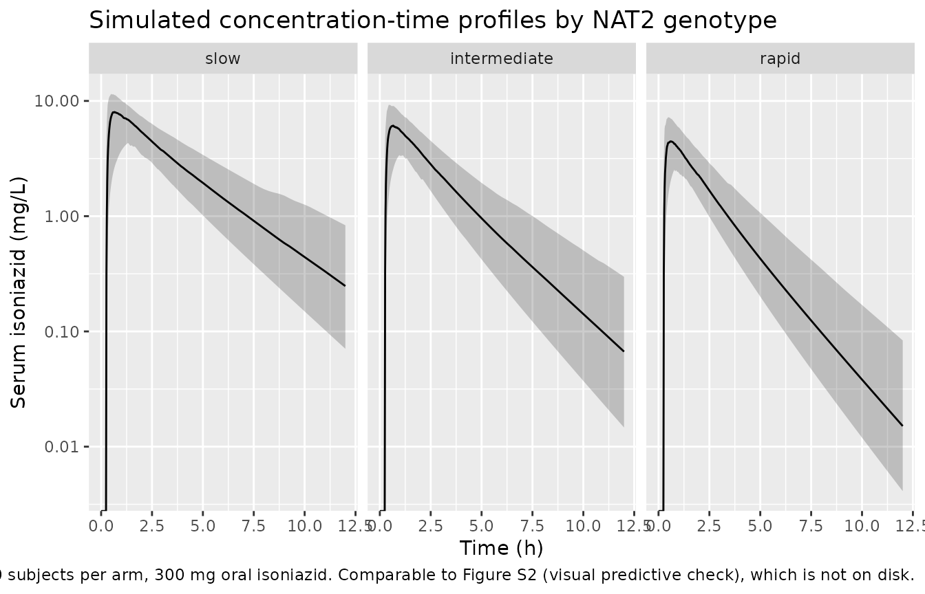

PKNCA validation

sim_nca <- sim |>
  dplyr::filter(!is.na(Cc)) |>
  dplyr::select(id, time, Cc, genotype)

# Guarantee a time = 0 row per subject; pre-dose Cc = 0 is correct for an
# extravascular dose.
sim_nca <- dplyr::bind_rows(
  sim_nca,
  sim_nca |> dplyr::distinct(id, genotype) |> dplyr::mutate(time = 0, Cc = 0)
) |>
  dplyr::distinct(id, genotype, time, .keep_all = TRUE) |>
  dplyr::arrange(id, genotype, time)

conc_obj <- PKNCA::PKNCAconc(sim_nca, Cc ~ time | genotype + id,
                             concu = "mg/L", timeu = "h")

dose_df <- events |>
  dplyr::filter(evid == 1) |>
  dplyr::select(id, time, amt, genotype)
dose_obj <- PKNCA::PKNCAdose(dose_df, amt ~ time | genotype + id, doseu = "mg")

intervals <- data.frame(
  start      = 0,
  end        = Inf,
  cmax       = TRUE,
  tmax       = TRUE,
  auclast    = TRUE,
  aucinf.obs = TRUE,
  half.life  = TRUE
)

nca_res <- PKNCA::pk.nca(PKNCA::PKNCAdata(conc_obj, dose_obj, intervals = intervals))

nca_tbl <- as.data.frame(nca_res$result)

# Confirm the gate has rows to test before summarising (a zero-row lookup would
# make every check below vacuously true).
stopifnot(
  all(c("cmax", "tmax", "aucinf.obs", "auclast", "half.life") %in% nca_tbl$PPTESTCD),
  sum(nca_tbl$PPTESTCD == "aucinf.obs" & !is.na(nca_tbl$PPORRES)) >=
    0.95 * 3 * n_per_arm
)

nca_med <- nca_tbl |>
  dplyr::filter(!is.na(PPORRES)) |>
  dplyr::group_by(genotype, PPTESTCD) |>
  dplyr::summarise(value = median(PPORRES), .groups = "drop") |>
  tidyr::pivot_wider(names_from = PPTESTCD, values_from = value)

# Reference side: Dose/CL is an identity for a linear model, so the
# typical-value AUC0-inf is a zero-parameter target; Cmax and Tmax come from
# the deterministic typical-value solve above.
published <- typ_summary |>
  dplyr::transmute(
    genotype   = as.character(genotype),
    cmax       = `Cmax (mg/L)`,
    tmax       = `Tmax (h)`,
    aucinf.obs = `AUC0-inf = Dose/CL (mg*h/L)`
  )

cmp <- nlmixr2lib::ncaComparisonTable(
  simulated = nca_res,
  reference = published,
  by        = "genotype",
  units     = c(cmax = "mg/L", tmax = "h", aucinf.obs = "mg*h/L"),
  tolerance_pct = 20
)

knitr::kable(cmp, digits = 2, align = c("l", "l", "r", "r", "r"),
             caption = paste("Simulated cohort medians against the typical-value",
                             "targets. * differs from reference by >20%."))

Simulated cohort medians against the typical-value targets. * differs from reference by >20%.

NCA parameter	genotype	Reference	Simulated	% diff
Cmax (mg/L)	slow	8.13	8.28	+1.9%
Cmax (mg/L)	intermediate	6.52	6.37	-2.3%
Cmax (mg/L)	rapid	4.98	4.81	-3.4%
Tmax (h)	slow	0.82	0.75	-8.5%
Tmax (h)	intermediate	0.7	0.68	-2.9%
Tmax (h)	rapid	0.6	0.6	+0.0%
AUC0-∞ (obs) (mg*h/L)	slow	27.3	28.4	+3.9%
AUC0-∞ (obs) (mg*h/L)	intermediate	16.7	17	+1.4%
AUC0-∞ (obs) (mg*h/L)	rapid	10.3	10	-2.7%

The AUC0-inf comparison is the load-bearing one: for a linear model AUC0-inf = Dose / (CL/F) is an identity, so a mis-transcribed clearance, dose or unit moves the simulated median by tens of percent. Cmax and Tmax are included for completeness but the cohort median of Cmax sits below the typical-value Cmax because the 139% CV on V/F makes the peak strongly right-skewed, and Tmax lands on a grid point.

auc_med <- nca_med |>
  dplyr::mutate(genotype = as.character(genotype)) |>
  dplyr::left_join(published, by = "genotype", suffix = c("", "_ref")) |>
  dplyr::mutate(auc_pct = 100 * (aucinf.obs - aucinf.obs_ref) / aucinf.obs_ref)

# Cohort-derived, so assert on the CENTRE rather than on any subject's extreme
# (see the repo CLAUDE.md note on thread-fragile assertions). Realised
# |auc_pct| was at most 3.9% across all three arms at 2 threads and 3.7% at 16;
# the residual is trapezoidal error on a peak that Tmax reaches in under an
# hour, not cohort noise. A bound of 12 leaves room for a different cohort draw
# while still breaking on a mis-transcribed clearance, dose or unit, which
# would move this by tens of percent.
stopifnot(
  max(abs(auc_med$auc_pct)) < 12,
  # Ordering of the three genotype AUCs is a structural claim with a 2.65-fold
  # spread, not a near-zero effect, so it is safe to assert.
  auc_med$aucinf.obs[auc_med$genotype == "slow"] >
    auc_med$aucinf.obs[auc_med$genotype == "intermediate"],
  auc_med$aucinf.obs[auc_med$genotype == "intermediate"] >
    auc_med$aucinf.obs[auc_med$genotype == "rapid"]
)

Immune activation drives the pre-ART to post-ART clearance change

The paper’s Figure 3 narrative is that isoniazid clearance rose after ART in most participants: “individual predicted isoniazid CL increased among three of five slow acetylators, five of nine intermediate acetylators and six of seven rapid acetylators” – 14 of 21, on a median %CD38+DR+CD8+ that fell from 36.9% to 24.8%. The IOV term is tiny (4.5% CV), so in this model the change is almost entirely the immune-activation covariate.

Simulating both occasions for the same subjects (common random numbers) turns this into a paired check.

set.seed(20170412)
rxode2::rxSetSeed(20170412)

n_paired <- 200L
cd38_sdlog_v2 <- log(35.9 / 21.9) / (2 * qnorm(0.75))

cd38_v1 <- draw_cd38(n_paired, cd38_ref, cd38_sdlog_v1)
cd38_v2 <- draw_cd38(n_paired, 24.8, cd38_sdlog_v2)

# One arm per occasion, intermediate genotype (the modal group), same subject
# IDs so etalcl is drawn once per subject per solve. Reseeding inside the loop
# gives common random numbers across the two occasions.
solve_occasion <- function(cd38, occ, seed) {
  rxode2::rxSetSeed(seed)
  ev <- make_events(genotypes[genotypes$genotype == "intermediate", ],
                    cd38 = cd38, occ = occ, n = n_paired)
  s <- rxode2::rxSolve(mod, ev, keep = "CD8_CD38DR_PCT", returnType = "data.frame")
  s <- s[!is.na(s$Cc), ]
  s |>
    dplyr::group_by(id) |>
    dplyr::summarise(cl = dplyr::first(cl),
                     cd38 = dplyr::first(CD8_CD38DR_PCT), .groups = "drop")
}

occ1 <- solve_occasion(cd38_v1, 1L, 991L)
occ2 <- solve_occasion(cd38_v2, 2L, 991L)

paired <- dplyr::inner_join(occ1, occ2, by = "id", suffix = c("_v1", "_v2")) |>
  dplyr::mutate(
    cl_ratio    = cl_v2 / cl_v1,
    cd38_ratio  = cd38_v2 / cd38_v1,
    # The model's analytic prediction for the ratio, ignoring the small IOV
    # term: (cd38_v2 / cd38_v1)^theta.
    predicted   = cd38_ratio^theta_cd38
  )

tibble::tibble(
  Quantity = c("Median CL/F, occasion 1 (L/h)",
               "Median CL/F, occasion 2 (L/h)",
               "Median CL/F ratio (occ 2 / occ 1)",
               "Ratio implied by the published medians, (24.8/36.9)^-0.31",
               "Fraction of subjects with higher CL/F after ART",
               "Vinnard 2017 Figure 3A: 14 of 21 participants"),
  Value = c(median(paired$cl_v1), median(paired$cl_v2),
            median(paired$cl_ratio), (24.8 / cd38_ref)^theta_cd38,
            mean(paired$cl_ratio > 1), 14 / 21)
) |>
  knitr::kable(digits = 3,
               caption = "Paired pre-ART / post-ART clearance change.")

Paired pre-ART / post-ART clearance change.

Quantity	Value
Median CL/F, occasion 1 (L/h)	18.350
Median CL/F, occasion 2 (L/h)	20.530
Median CL/F ratio (occ 2 / occ 1)	1.125
Ratio implied by the published medians, (24.8/36.9)^-0.31	1.131
Fraction of subjects with higher CL/F after ART	0.750
Vinnard 2017 Figure 3A: 14 of 21 participants	0.667

rel_err <- abs(paired$cl_ratio / paired$predicted - 1)

# Every bound below is set from the ANALYTIC expectation, not from one run.
# The only quantity separating cl_ratio from its covariate-only prediction is
# the IOV term, whose difference across two occasions has SD
# 0.045 * sqrt(2) = 0.064, giving an expected median |rel_err| of 0.043 and an
# expected 90th percentile of 0.105 (realised 0.042 and 0.104 at 2 threads).
# The bounds sit at roughly twice those, so they break if the covariate form is
# wrong (rel_err would then be systematically tens of percent) or if the IOV
# variance were mis-transcribed by a factor of two -- but not on a cohort draw.
stopifnot(
  median(rel_err) < 0.08,
  quantile(rel_err, 0.9) < 0.20,
  # A majority of subjects clear faster after ART, as in Figure 3A. The
  # analytic fraction is 0.76 (realised 0.75); the published fraction is
  # 14/21 = 0.67. Asserting > 0.55 needs the whole mean shift to vanish.
  mean(paired$cl_ratio > 1) > 0.55,
  # The median ratio tracks the ratio implied by the published visit medians;
  # analytic agreement is exact, realised relative error 0.006 at 2 threads.
  abs(median(paired$cl_ratio) / ((24.8 / cd38_ref)^theta_cd38) - 1) < 0.12
)

Assumptions and deviations

• Covariate functional forms are not printed by the paper. Table 2 gives three coefficients and no equation. The proportional (1 + theta) form for NAT2 and the median-normalised power form for %CD38+DR+CD8+ were identified from four published anchors (Figure 3A per-genotype clearances, Figure 2A base-model etas, the Results BSV-reduction sequence, and the Figure 2B regression slope) plus an external cross-check against Horita_2018_isoniazid. All are shown above with the rejected alternatives side by side. This is the single largest interpretive step in the extraction: a reader who has access to the authors’ Phoenix NLME control stream should check it against the forms above.
• The normalising value for %CD38+DR+CD8+ (36.9%) is the visit-1 cohort median from Table 1, not a value the paper identifies as the normalisation constant. The model was fit to both occasions pooled, so the constant the authors actually used was most likely the pooled median (somewhere between the 36.9% visit-1 and 24.8% visit-2 medians). Using 36.9% makes lcl exactly the printed 10.99 L/h at visit-1-median activation; a different constant would rescale lcl by (constant / 36.9)^-0.31 and leave every prediction in this vignette unchanged in shape.
• Non-paper-derived values used for validation only. The Figure 2A eta medians (-0.53 / 0.07 / 0.40), the Figure 2B regression endpoints (+0.225 at x = 9.5, -0.29 at x = 66.5), the Figure 3A clearance medians (10.2 / 19.0 / 26.5 L/h) and the Figure 3B AUC medians (28.5 / 15.2 / 11.0 mg*h/L) were read off the published figures by on-screen digitisation, with roughly +/- 10% uncertainty. No ini() parameter value comes from a figure – every one is a printed Table 2 estimate.
• Isoniazid dose is not tabulated. The paper states only that participants were dosed by WHO weight band. For a linear model AUC0-inf = Dose / (CL/F), so pairing the Figure 3A clearances with the Figure 3B AUCs for the slow acetylators back-solves the dose: the six recoverable pairs give 278 to 343 mg with a mean of 302 mg. The simulations here therefore use 300 mg, which is also the standard adult isoniazid component of the WHO 55-70 kg band that contains this cohort’s median weight of 55.0 kg. The companion paper on the same cohort (Vinnard 2017, J Antimicrob Chemother, Vinnard_2017_rifampicin) reports rifampicin doses of 300/450/600/750 mg for 1/19/17/3 participants, i.e. 2/3/4/5 tablets of the same fixed-dose combination, implying isoniazid doses of 150/225/300/375 mg across the cohort.
• BSV reported as a percentage is read as CV% and converted with the exact log-normal identity omega^2 = log(1 + CV^2). The paper says only that BSV used “an exponential variability model with mean of zero and variance omega^2” and tabulates percentages. This matters most for BSV-V at 139.3%, where omega = 1.039 under this identity versus 1.393 if the percentage were read as omega * 100.
• Inter-occasion variability is encoded as two etas with equal variance. Table 2 reports one IOV variance (4.5% CV) shared across the two occasions, which in NONMEM would be $OMEGA BLOCK(1) plus SAME. nlmixr2 has no SAME shortcut, so the second occasion’s variance is fixed equal to the first – the pattern used by Wilkins_2008_rifampicin and the companion Vinnard_2017_rifampicin. rxode2 warns that these indicator-multiplexed etas are not mu-referenced; that is expected for the IOV idiom and does not affect simulation.
• The two ambiguous-NAT2 participants are not representable. The paper resolved 38 of 40 genotypes and does not say how the other two entered the covariate model. Set NAT2_SLOW = 0, NAT2_RAPID = 0 to place a subject in the intermediate group, or exclude them.
• Screened-and-rejected covariates carry no coefficients. Creatinine clearance, sex, weight, CD4+ count, IL-6, neopterin and CRP were all tested and none was retained; the paper reports no point estimates for them, so they are documented in the model file’s covariatesDataExcluded list rather than in covariateData. In particular there is no allometric weight scaling in this model, which is why the Horita_2018_isoniazid cross-check above has to supply the 0.75 exponent externally.
• The supplement is not obtainable and is not needed. Europe PMC reports Article with id PMC5346858 is not open access one for the supplementary-file endpoint (a control PMCID returned a valid archive from the same endpoint, so this is a missing deposit rather than a service outage). The supplement holds Table S1 (per-participant NAT2 alleles), Table S2 (NAT2 gene positions), Figure S1 (goodness-of-fit plots) and Figure S2 (visual predictive checks) – no parameter estimates. Every ini() value comes from Table 2 of the main article, so no parameter is missing. The absent Figure S2 is the one validation target that could not be reproduced directly; the simulated profiles above stand in for it.
• V/F is weakly identified in the source. Table 2 reports V = 5.55 L with 48% RSE, a bootstrap 95% CI of 2.01 to 12.31 L, and 139.3% BSV. Reproduced faithfully, this makes the simulated peak concentration strongly right-skewed and the typical-value Cmax (about 8 mg/L at 300 mg in a slow acetylator) higher than the cohort median. The paper’s sampling schedule has no observation between 0.3 and 0.9 h, which brackets this model’s Tmax, so the peak is the least-constrained region of the fit. Exposure metrics (AUC0-inf, and therefore the paper’s own conclusions) depend only on CL/F and are unaffected.