Atogepant (Schlachter 2026)
Source:vignettes/articles/Schlachter_2026_atogepant.Rmd
Schlachter_2026_atogepant.RmdModel and source
- Citation: Schlachter L, Stodtmann S, Voelkner A, Jonsson F, Lagraauw HM, Boinpally RR. Population Pharmacokinetics of Atogepant for the Prevention of Migraine. Clin Pharmacokinet. 2026;65(2):151-166. doi:10.1007/s40262-025-01566-5.
- Description: Three-compartment population pharmacokinetic model for oral atogepant, a calcitonin gene-related peptide (CGRP) receptor antagonist for the preventive treatment of migraine, pooled across 12 phase 1 studies, 1 phase 2b/3 study and 1 phase 3 study in healthy participants and patients with episodic migraine (Schlachter 2026 ‘Phase 3 Model’). Absorption is sequential zero-order into the depot over a duration Tk0 followed by a first-order transfer ka into the central compartment, the whole input delayed by an absorption lag time; ka is not estimated independently but is derived from Tk0 and the estimated zero-order time fraction Fk0. Apparent clearance is lower in migraine patients than in healthy participants and is modified by severe hepatic impairment, itraconazole, quinidine and single- versus multiple-dose rifampicin; apparent central volume increases with body weight; relative bioavailability increases with dose and is modified by itraconazole and rifampicin; a high-fat meal lengthens the lag time; and the zero-order duration depends on dose and on the early phase 1 tablet formulation. Residual error is proportional with four study-specific magnitudes, and a blood-to-plasma ratio converts the plasma prediction to the dried-blood-sample matrix.
- Article: https://doi.org/10.1007/s40262-025-01566-5
- Supplement: https://doi.org/10.1007/s40262-025-01566-5 (Supplementary Information, open access)
Atogepant (Qulipta / Aquipta) is an oral calcitonin gene-related peptide (CGRP) receptor antagonist approved for the preventive treatment of episodic and chronic migraine. Schlachter 2026 reports the population pharmacokinetic model that supported dose selection and the regulatory filings, developed in three stages across the programme. This vignette packages the Phase 3 Model, the final model of the paper; the Phase 1 and Phase 2 Models are earlier development iterations of the same analysis and are superseded by it, so per the library’s replicate-the-author’s-structure policy only the final model is extracted.
Population
The Phase 3 Model was fitted to 11,763 atogepant concentrations from 1356 participants: 351 healthy participants from 12 phase 1 studies, 463 patients with episodic migraine from the phase 2b/3 study CGP-MD-01, and 542 patients with episodic migraine from the pivotal phase 3 ADVANCE study (Table 1 and supplementary Tables S1 and S2). Median age was 39 years (range 18 to 78), median body weight 77.6 kg (40.7 to 196), and 74.7% were female. The population was 76.0% Caucasian, 17.9% Black or African American and 3.5% Asian. Hepatic function was normal in 98.2%, with 8 subjects in each of the mild, moderate and severe strata contributed by the dedicated hepatic-impairment study CGP-PK-01. Renal function was normal in 87.2%, mildly impaired in 11.9% and moderately impaired in 1.0%; no subject had severe renal impairment. Concomitant medications of interest were itraconazole (40 subjects), rifampicin (31) and quinidine (25), each from a dedicated drug-drug-interaction study, plus concomitant statins in 67 subjects.
The model was then externally validated without re-estimation against 350 patients with chronic migraine (PROGRESS) and 127 patients with episodic migraine for whom two to four classes of conventional oral preventive treatments had failed (ELEVATE). Those 477 subjects are not part of the 1356 above.
The same information is available programmatically via the model’s
population metadata:
pop <- rxode2::rxode(readModelDb("Schlachter_2026_atogepant"))$population
#> ℹ parameter labels from comments will be replaced by 'label()'
#> Warning: some etas defaulted to non-mu referenced, possible parsing error: etaiov_fdepot_1, etaiov_fdepot_2, etaiov_fdepot_3, etaiov_fdepot_4
#> as a work-around try putting the mu-referenced expression on a simple line
str(pop, max.level = 1)
#> List of 15
#>  $ species       : chr "human"
#>  $ n_subjects    : num 1356
#>  $ n_studies     : num 14
#>  $ age_range     : chr "18-78 years"
#>  $ age_median    : chr "39.0 years"
#>  $ weight_range  : chr "40.7-196 kg"
#>  $ weight_median : chr "77.6 kg"
#>  $ height_median : chr "166 cm (range 146-204)"
#>  $ sex_female_pct: num 74.7
#>  $ race_ethnicity: Named num [1:7] 76 17.9 3.5 1.9 0.3 0.2 0.1
#>   ..- attr(*, "names")= chr [1:7] "Caucasian" "Black/African American" "Asian" "Multiple" ...
#>  $ disease_state : chr "351 healthy participants and 1005 patients with episodic migraine. Hepatic function: 98.2% none, 0.6% mild, 0.6"| __truncated__
#>  $ renal_function: chr "median creatinine clearance 127 mL/min (range 46.5-392)"
#>  $ co_medication : chr "Itraconazole 40 subjects (2.9%), rifampicin 31 (2.3%), quinidine 25 (1.8%), concomitant statin 67 (4.9%); 1260 "| __truncated__
#>  $ dose_range    : chr "10-300 mg oral tablet, once or twice daily, single and multiple dose"
#>  $ notes         : chr "Baseline characteristics from Schlachter 2026 Table 1, Phase 3 Model column. 11,763 observations from 1356 part"| __truncated__
Model structure
Three disposition compartments with linear elimination from the
central compartment, and a sequential zero-order then
first-order absorption process with a lag time. The
bioavailable dose is released into the depot at a zero-order rate over a
duration Tk0, and the depot empties into the central
compartment at first-order rate ka, with the whole input
delayed by ALAG.
ka is not estimated independently. Section 3.1 states it
“was linked to the zero-order input parameters through
ka = Fk0 / [Tk0 * (1 - Fk0)]”, which rearranges exactly to
Fk0 = Tk0 / (Tk0 + 1/ka): Fk0 is the fraction
of the total absorption time constant contributed by
the zero-order step, not (as the surrounding prose loosely glosses it) a
fraction of the dose. The consequence matters for the covariate model:
because dose and formulation are applied to Tk0, they
propagate into ka, which is why Table 2 labels those two
estimates as effects “on ka” while the display equations apply them to
Tk0.
ui <- rxode2::rxode(readModelDb("Schlachter_2026_atogepant"))
#> ℹ parameter labels from comments will be replaced by 'label()'
#> Warning: some etas defaulted to non-mu referenced, possible parsing error: etaiov_fdepot_1, etaiov_fdepot_2, etaiov_fdepot_3, etaiov_fdepot_4
#> as a work-around try putting the mu-referenced expression on a simple line
cat("ODE states :", paste(ui$state, collapse = ", "), "\n")
#> ODE states : depot, central, peripheral1, peripheral2
cat("Covariates :", paste(sort(ui$allCovs), collapse = ", "), "\n")
#> Covariates : CONMED_ITRACONAZOLE, CONMED_QUINIDINE, CONMED_RIFAMPICIN_MD, CONMED_RIFAMPICIN_SD, DIS_HEALTHY, DOSE_ATOGEPANT_MG, FED_HIGHFAT, FORM_ATOGEPANT_EARLYTAB, HEPIMP_SEV, OCC, STUDY_ATOGEPANT_PHASE3, STUDY_CGP_MD_01, STUDY_CGP_PK_02, WT
Source trace
Every ini() entry in
inst/modeldb/specificDrugs/Schlachter_2026_atogepant.R
carries an in-file comment naming its source location. They are
collected here for review. “Eq.” refers to the unnumbered display
equations printed in Section 3.1 of the paper.
| Equation / parameter | Value | Source location |
|---|---|---|
lcl (CL/F, patients) |
17.4 L/h | Table 2, “Apparent clearance patients” (RSE 2%) |
lvc (V1/F) |
86.1 L | Table 2, “Apparent central volume of distribution” (RSE 2.3%) |
lq (Q/F) |
1.43 L/h | Table 2, “Apparent first intercompartmental clearance” (RSE 10%) |
lvp (V2/F) |
40.5 L | Table 2, “Apparent first peripheral volume of distribution” (RSE 7.3%) |
lq2 (Q2/F) |
1.68 L/h | Table 2, “Apparent second intercompartmental clearance” (RSE 7.4%) |
lvp2 (V3/F) |
13.0 L | Table 2, “Apparent second peripheral volume of distribution” (RSE 11.9%) |
ld1 (Tk0) |
0.908 h | Table 2, “Duration zero-order absorption” (RSE 4.7%) |
ltlag (ALAG) |
0.276 h | Table 2, “Lag time” (RSE 0.5%) |
fzo (Fk0) |
0.693 | Table 2, “Fraction zero-order absorption” (RSE 2.9%) |
lfdepot (Frel at 60 mg) |
1 (fixed) | Sect. 3.1 Frel Eq.; Frel is purely relative, anchored at the 60 mg reference |
bpr |
0.573 | Table 2, “Blood-plasma ratio” (RSE 2%) |
e_dis_healthy_cl |
0.3161 | Derived from the two Table 2 typical values: 22.9 / 17.4 - 1 |
e_hepimp_sev_cl |
-0.366 | Table 2, “Effect of severe hepatic impairment on CL/F”; Sect. 3.1 CL/F Eq. |
e_conmed_itraconazole_cl |
-0.662 | Table 2, “Itraconazole effect on CL/F”; Sect. 3.1 CL/F Eq. |
e_conmed_quinidine_cl |
-0.285 | Table 2, “Quinidine effect on CL/F”; Sect. 3.1 CL/F Eq. |
e_conmed_rifampicin_sd_cl |
-0.128 | Table 2, “Rifampin effect on CL/F after first dose” |
e_conmed_rifampicin_md_cl |
0.818 | Table 2, “Rifampin effect on CL/F following multiple doses” |
e_wt_vc |
0.411 | Table 2, “Exponential weight effect on V1/F”; Sect. 3.1 V1/F Eq. (76.8 kg reference) |
e_dose_atogepant_mg_fdepot |
0.119 | Table 2, “Exponential dose effect on Frel”; Sect. 3.1 Frel Eq. (60 mg reference) |
e_conmed_itraconazole_fdepot |
0.949 | Table 2, “Itraconazole effect on Frel” |
e_conmed_rifampicin_sd_fdepot |
1.42 | Table 2, “Rifampin effect on Frel after first dose” |
e_conmed_rifampicin_md_fdepot |
-0.248 | Table 2, “Rifampin effect on Frel following multiple doses” |
e_fed_highfat_tlag |
0.672 | Table 2, “Food effect on ALAG”; Sect. 3.1 ALAG Eq. |
e_dose_atogepant_mg_d1 |
0.199 | Table 2 (labelled “on ka”); Sect. 3.1 Tk0 Eq. applies it to Tk0 |
e_form_atogepant_earlytab_d1 |
-0.353 | Table 2 (labelled “on ka”); Sect. 3.1 Tk0 Eq. applies it to Tk0 |
etalcl |
0.0243 | Table 2, “omega2 CL/F”; sqrt = 15.6% CV, matching Sect. 3.1 |
etald1 |
0.163 | Table 2, “omega2 tk0”; sqrt = 40.4% CV |
etalfdepot |
0.234 | Table 2, “omega2 Frel”; sqrt = 48.4% CV |
etalq / etalvp block |
0.471 / 0.422 / 0.601 | Table 2, “omega2 Q/F”, “Cov Q/F,V2/F”, “omega2 V2/F”; sqrt of diagonals = 68.6% and 77.5% CV |
etaiov_fdepot_* |
0.0373 | Table 2, “omega IOV Frel”; sqrt = 19.3% CV |
propSdPhase1 |
0.307 | Table 2, “sigma prop”; 30.7% CV |
propSdCgpPk02 |
0.228 | Table 2, “sigma prop (study CGP-PK-02)”; 22.8% CV |
propSdCgpMd01 |
0.585 | Table 2, “sigma prop (study CGP-MD-01)”; 58.5% CV |
propSdPhase3 |
0.491 | Table 2, “sigma prop (ADVANCE and PROGRESS studies)”; 49.1% CV |
| ODE system (3 compartments, linear elimination) | n/a | Sect. 3.2.1 and the Discussion |
ka = Fk0 / (Tk0 * (1 - Fk0)) |
n/a | Sect. 3.1, verbatim |
Concentration scaling (* 1000) |
n/a | Units: mg dose / L volume gives mg/L; the paper reports ng/mL |
Deterministic structural checks
These compare quantities the paper states in prose against the packaged model’s own arithmetic. They are deterministic – no simulated cohort is involved – so the tolerances are tight and are expected to stay tight.
th <- ui$theta

# Fk0 / Tk0 / ka relationship, Sect. 3.1.
tk0_ref <- exp(th[["ld1"]])
fzo_ref <- th[["fzo"]]
ka_derived <- fzo_ref / (tk0_ref * (1 - fzo_ref))

# Frel ratio between the 60 mg and 10 mg doses, Sect. 3.1 / Discussion.
frel_ratio_60_10 <- (60 / 60)^th[["e_dose_atogepant_mg_fdepot"]] /
  (10 / 60)^th[["e_dose_atogepant_mg_fdepot"]]

# Lag time after a high-fat meal, Sect. 3.1.
alag_fed <- exp(th[["ltlag"]]) * (1 + th[["e_fed_highfat_tlag"]])

# Tk0 shortening for the early phase 1 tablet, Sect. 3.1.
tk0_pct_shorter <- -100 * th[["e_form_atogepant_earlytab_d1"]]

# Healthy-participant clearance recovered from the patient typical value.
cl_healthy <- exp(th[["lcl"]]) * (1 + th[["e_dis_healthy_cl"]])

structural <- tibble::tribble(
  ~Quantity,                                  ~Published, ~Model,
  "Derived ka (1/h)",                          2.48,       ka_derived,
  "Frel ratio, 60 mg vs 10 mg",                1.24,       frel_ratio_60_10,
  "Lag time after a high-fat meal (h)",        0.46,       alag_fed,
  "Tk0 shortening, early phase 1 tablet (%)", 35.0,        tk0_pct_shorter,
  "CL/F in healthy participants (L/h)",       22.9,        cl_healthy,
  "Blood-to-plasma ratio",                     0.573,      th[["bpr"]]
) |>
  mutate(`Diff (%)` = 100 * (Model - Published) / Published)

knitr::kable(structural, digits = 3,
caption = "Model arithmetic vs values stated in Schlachter 2026 Section 3.1.")| Quantity | Published | Model | Diff (%) |
|---|---|---|---|
| Derived ka (1/h) | 2.480 | 2.486 | 0.244 |
| Frel ratio, 60 mg vs 10 mg | 1.240 | 1.238 | -0.189 |
| Lag time after a high-fat meal (h) | 0.460 | 0.461 | 0.320 |
| Tk0 shortening, early phase 1 tablet (%) | 35.000 | 35.300 | 0.857 |
| CL/F in healthy participants (L/h) | 22.900 | 22.900 | 0.001 |
| Blood-to-plasma ratio | 0.573 | 0.573 | 0.000 |
# Each published figure is rounded to 2-3 significant figures, so 1% is ample
# headroom for rounding while still catching a mis-transcribed estimate (which
# would move these by tens of percent).
stopifnot(max(abs(structural$`Diff (%)`)) < 1)
Interindividual variability on the reported CV scale
Table 2 reports variances; the Table 1 footnote states that IIV is
derived as sqrt(omega^2) * 100. Recomputing the percent CVs
quoted in Section 3.1 from the packaged variances confirms the scale
(variance, not SD) was read correctly.
om <- ui$omega
iiv <- tibble::tribble(
  ~Parameter,        ~Variance,               ~`Published CV (%)`,
  "CL/F",             om["etalcl", "etalcl"],         15.6,
  "Tk0",              om["etald1", "etald1"],         40.4,
  "Frel",             om["etalfdepot", "etalfdepot"], 48.4,
  "Q/F",              om["etalq", "etalq"],           68.6,
  "V2/F",             om["etalvp", "etalvp"],         77.5,
  "Frel (IOV)",       om["etaiov_fdepot_1", "etaiov_fdepot_1"], 19.3
) |>
  mutate(`Model CV (%)` = 100 * sqrt(Variance),
         `Diff (%)` = 100 * (`Model CV (%)` - `Published CV (%)`) / `Published CV (%)`)

knitr::kable(iiv, digits = 3,
caption = "IIV variances back-transformed to the percent CVs quoted in Section 3.1.")| Parameter | Variance | Published CV (%) | Model CV (%) | Diff (%) |
|---|---|---|---|---|
| CL/F | 0.024 | 15.6 | 15.588 | -0.074 |
| Tk0 | 0.163 | 40.4 | 40.373 | -0.066 |
| Frel | 0.234 | 48.4 | 48.374 | -0.055 |
| Q/F | 0.471 | 68.6 | 68.629 | 0.043 |
| V2/F | 0.601 | 77.5 | 77.524 | 0.031 |
| Frel (IOV) | 0.037 | 19.3 | 19.313 | 0.068 |
stopifnot(max(abs(iiv$`Diff (%)`)) < 0.5)

# The Q/F - V2/F covariance implies a strong positive correlation.
cor_q_vp <- om["etalq", "etalvp"] / sqrt(om["etalq", "etalq"] * om["etalvp", "etalvp"])
cat(sprintf("Implied Q/F - V2/F correlation: %.3f\n", cor_q_vp))
#> Implied Q/F - V2/F correlation: 0.793
stopifnot(cor_q_vp > 0.7, cor_q_vp < 0.9)
Mass-balance check on the ODE system
For a linear model the total exposure after a single dose is exactly
Dose * Frel / (CL/F), independent of the absorption and
distribution structure. Reproducing that identity from the solved ODE
system confirms the compartment wiring, the bioavailability target, and
the mg-to-ng/mL scaling simultaneously. Because both sides use the same
drawn parameters, the only difference is numerical-integration error and
the bound is correspondingly tight.
mod  <- readModelDb("Schlachter_2026_atogepant")
modT <- rxode2::zeroRe(mod)
#> ℹ parameter labels from comments will be replaced by 'label()'
#> Warning: some etas defaulted to non-mu referenced, possible parsing error: etaiov_fdepot_1, etaiov_fdepot_2, etaiov_fdepot_3, etaiov_fdepot_4
#> as a work-around try putting the mu-referenced expression on a simple line
#> Warning: No sigma parameters in the model
#> Warning: some etas defaulted to non-mu referenced, possible parsing error: etaiov_fdepot_1, etaiov_fdepot_2, etaiov_fdepot_3, etaiov_fdepot_4
#> as a work-around try putting the mu-referenced expression on a simple line

# Reference covariate set: a typical migraine patient at the population median
# weight, Formulation 5, fasted, no interacting comedication, phase 3 study.
base_covs <- list(
  OCC = 1, DIS_HEALTHY = 0, HEPIMP_SEV = 0, CONMED_ITRACONAZOLE = 0,
  CONMED_QUINIDINE = 0, CONMED_RIFAMPICIN_SD = 0, CONMED_RIFAMPICIN_MD = 0,
  WT = 77.6, DOSE_ATOGEPANT_MG = 60, FORM_ATOGEPANT_EARLYTAB = 0,
  FED_HIGHFAT = 0, STUDY_CGP_PK_02 = 0, STUDY_CGP_MD_01 = 0,
  STUDY_ATOGEPANT_PHASE3 = 1
)

# `rate = -2` tells rxode2 to use the model's own dur(depot) for the
# zero-order input rather than treating the record as a bolus.
solve_typical <- function(dose, times, covs = list(), ii = NULL, until = NULL) {
  cv <- modifyList(base_covs, c(list(DOSE_ATOGEPANT_MG = dose), covs))
  ev <- if (is.null(ii)) {
    rxode2::et(amt = dose, cmt = "depot", rate = -2)
  } else {
    rxode2::et(amt = dose, cmt = "depot", rate = -2, ii = ii, until = until)
  }
  # Observation rows point at the ODE state `central`; rxode2 returns the
  # algebraic observables Cc and Cb as columns at those rows.
  ev <- rxode2::et(ev, times, cmt = "central")
  d <- as.data.frame(ev)
  for (nm in names(cv)) d[[nm]] <- cv[[nm]]
  rxode2::rxSolve(modT, d, returnType = "data.frame") |>
    dplyr::filter(!is.na(Cc))
}

trap_auc <- function(time, conc) {
  sum(diff(time) * (utils::head(conc, -1) + utils::tail(conc, -1)) / 2)
}

# 21 days is many multiples of the ~11 h terminal half-life, so the truncated
# AUC is within rounding of AUC(0, Inf).
sd_grid <- sort(unique(c(seq(0, 24, by = 0.02), seq(24, 504, by = 0.5))))
mb <- lapply(c(10, 30, 60), function(d) {
  s <- solve_typical(d, sd_grid)
  frel <- (d / 60)^ui$theta[["e_dose_atogepant_mg_fdepot"]]
  tibble::tibble(
    Dose = paste(d, "mg"),
    `AUC from ODE (ng*h/mL)` = trap_auc(s$time, s$Cc),
    `Dose * Frel / (CL/F)`   = d * frel / exp(ui$theta[["lcl"]]) * 1000
  )
}) |> bind_rows() |>
  mutate(`Diff (%)` = 100 * (`AUC from ODE (ng*h/mL)` - `Dose * Frel / (CL/F)`) /
           `Dose * Frel / (CL/F)`)
#> ℹ omega/sigma items treated as zero: 'etalcl', 'etald1', 'etalfdepot', 'etalq', 'etalvp', 'etaiov_fdepot_1', 'etaiov_fdepot_2', 'etaiov_fdepot_3', 'etaiov_fdepot_4'
#> ℹ omega/sigma items treated as zero: 'etalcl', 'etald1', 'etalfdepot', 'etalq', 'etalvp', 'etaiov_fdepot_1', 'etaiov_fdepot_2', 'etaiov_fdepot_3', 'etaiov_fdepot_4'
#> ℹ omega/sigma items treated as zero: 'etalcl', 'etald1', 'etalfdepot', 'etalq', 'etalvp', 'etaiov_fdepot_1', 'etaiov_fdepot_2', 'etaiov_fdepot_3', 'etaiov_fdepot_4'

knitr::kable(mb, digits = 2,
caption = "Single-dose mass balance: solved AUC vs the closed-form identity.")| Dose | AUC from ODE (ng*h/mL) | Dose * Frel / (CL/F) | Diff (%) |
|---|---|---|---|
| 10 mg | 464.36 | 464.36 | 0 |
| 30 mg | 1587.64 | 1587.63 | 0 |
| 60 mg | 3448.30 | 3448.28 | 0 |
Covariate-effect replication
Every intrinsic and extrinsic factor the paper retained is exercised here by solving the packaged model with and without the covariate set and comparing the realised exposure ratio against the ratio implied by the published coefficients. This is the check that the covariate wiring – which parameter each effect lands on, and in which direction – is correct. It is deterministic, so the tolerance is tight.
# AUC ratio implied by the published coefficients: a factor on Frel raises
# exposure, a factor on CL/F lowers it.
scenarios <- tibble::tribble(
  ~Scenario,                       ~covs,                                  ~cl_fac, ~frel_fac,
  "Healthy vs migraine patient",   list(DIS_HEALTHY = 1),                   1.3161,   1,
  "Severe hepatic impairment",     list(HEPIMP_SEV = 1),                    1 - 0.366, 1,
  "Itraconazole",                  list(CONMED_ITRACONAZOLE = 1),           1 - 0.662, 1 + 0.949,
  "Quinidine",                     list(CONMED_QUINIDINE = 1),              1 - 0.285, 1,
  "Rifampicin, single dose",       list(CONMED_RIFAMPICIN_SD = 1),          1 - 0.128, 1 + 1.42,
  "Rifampicin, multiple doses",    list(CONMED_RIFAMPICIN_MD = 1),          1 + 0.818, 1 - 0.248
)

ref <- solve_typical(60, sd_grid)
#> ℹ omega/sigma items treated as zero: 'etalcl', 'etald1', 'etalfdepot', 'etalq', 'etalvp', 'etaiov_fdepot_1', 'etaiov_fdepot_2', 'etaiov_fdepot_3', 'etaiov_fdepot_4'
auc_ref <- trap_auc(ref$time, ref$Cc)

cov_tab <- lapply(seq_len(nrow(scenarios)), function(i) {
  s <- solve_typical(60, sd_grid, covs = scenarios$covs[[i]])
  tibble::tibble(
    Scenario = scenarios$Scenario[i],
    `Expected AUC ratio` = scenarios$frel_fac[i] / scenarios$cl_fac[i],
    `Simulated AUC ratio` = trap_auc(s$time, s$Cc) / auc_ref
  )
}) |> bind_rows() |>
  mutate(`Diff (%)` = 100 * (`Simulated AUC ratio` - `Expected AUC ratio`) /
           `Expected AUC ratio`)
#> ℹ omega/sigma items treated as zero: 'etalcl', 'etald1', 'etalfdepot', 'etalq', 'etalvp', 'etaiov_fdepot_1', 'etaiov_fdepot_2', 'etaiov_fdepot_3', 'etaiov_fdepot_4'
#> ℹ omega/sigma items treated as zero: 'etalcl', 'etald1', 'etalfdepot', 'etalq', 'etalvp', 'etaiov_fdepot_1', 'etaiov_fdepot_2', 'etaiov_fdepot_3', 'etaiov_fdepot_4'
#> ℹ omega/sigma items treated as zero: 'etalcl', 'etald1', 'etalfdepot', 'etalq', 'etalvp', 'etaiov_fdepot_1', 'etaiov_fdepot_2', 'etaiov_fdepot_3', 'etaiov_fdepot_4'
#> ℹ omega/sigma items treated as zero: 'etalcl', 'etald1', 'etalfdepot', 'etalq', 'etalvp', 'etaiov_fdepot_1', 'etaiov_fdepot_2', 'etaiov_fdepot_3', 'etaiov_fdepot_4'
#> ℹ omega/sigma items treated as zero: 'etalcl', 'etald1', 'etalfdepot', 'etalq', 'etalvp', 'etaiov_fdepot_1', 'etaiov_fdepot_2', 'etaiov_fdepot_3', 'etaiov_fdepot_4'
#> ℹ omega/sigma items treated as zero: 'etalcl', 'etald1', 'etalfdepot', 'etalq', 'etalvp', 'etaiov_fdepot_1', 'etaiov_fdepot_2', 'etaiov_fdepot_3', 'etaiov_fdepot_4'

knitr::kable(cov_tab, digits = 3,
             caption = paste(
               "Covariate effects on single-dose AUC, relative to a typical",
               "migraine patient with no interacting comedication."
))| Scenario | Expected AUC ratio | Simulated AUC ratio | Diff (%) |
|---|---|---|---|
| Healthy vs migraine patient | 0.760 | 0.760 | 0.000 |
| Severe hepatic impairment | 1.577 | 1.577 | 0.001 |
| Itraconazole | 5.766 | 5.766 | 0.000 |
| Quinidine | 1.399 | 1.399 | 0.000 |
| Rifampicin, single dose | 2.775 | 2.775 | 0.000 |
| Rifampicin, multiple doses | 0.414 | 0.414 | -0.001 |
The paper describes these same effects in words in Section 3.1 and the Discussion: itraconazole and quinidine lower CL/F by 66.2% and 28.5%; itraconazole raises Frel 1.95-fold; a single rifampicin dose raises Frel 2.4-fold and lowers CL/F by 12.8%, while multiple rifampicin doses raise CL/F 1.82-fold and lower Frel by 24.8%; severe hepatic impairment lowers CL/F by 36.6%. The table above confirms each lands on the right parameter with the right sign, and shows the net exposure consequence – most strikingly the 5.8-fold AUC increase with itraconazole, which combines the clearance and bioavailability effects in the same direction.
Body weight acts on V1/F alone, so it shifts Cmax without changing AUC:
wt_tab <- lapply(c(50, 77.6, 120), function(w) {
  s <- solve_typical(60, sd_grid, covs = list(WT = w))
  tibble::tibble(`Body weight (kg)` = w,
                 `Cmax (ng/mL)` = max(s$Cc),
                 `AUC (ng*h/mL)` = trap_auc(s$time, s$Cc))
}) |> bind_rows()
#> ℹ omega/sigma items treated as zero: 'etalcl', 'etald1', 'etalfdepot', 'etalq', 'etalvp', 'etaiov_fdepot_1', 'etaiov_fdepot_2', 'etaiov_fdepot_3', 'etaiov_fdepot_4'
#> ℹ omega/sigma items treated as zero: 'etalcl', 'etald1', 'etalfdepot', 'etalq', 'etalvp', 'etaiov_fdepot_1', 'etaiov_fdepot_2', 'etaiov_fdepot_3', 'etaiov_fdepot_4'
#> ℹ omega/sigma items treated as zero: 'etalcl', 'etald1', 'etalfdepot', 'etalq', 'etalvp', 'etaiov_fdepot_1', 'etaiov_fdepot_2', 'etaiov_fdepot_3', 'etaiov_fdepot_4'

knitr::kable(wt_tab, digits = 1,
caption = "Body weight acts on V1/F only: Cmax moves, AUC does not.")| Body weight (kg) | Cmax (ng/mL) | AUC (ng*h/mL) |
|---|---|---|
| 50.0 | 614.7 | 3448.3 |
| 77.6 | 531.8 | 3448.3 |
| 120.0 | 458.9 | 3448.3 |
# AUC must be analytically identical across weights (weight touches no
# clearance term); the residual spread is trapezoidal discretisation error,
# which grows slightly as the peak sharpens at low weight. Realised 5.0e-6
# (3448.296 / 3448.304 / 3448.313, i.e. agreement to 7 significant figures);
# 1e-4 leaves two orders of magnitude of headroom while still catching a
# weight term leaking into a clearance parameter, which would be percent-level.
# Both checks are deterministic -- no cohort is drawn -- so the bounds are tight.
stopifnot(diff(range(wt_tab$`AUC (ng*h/mL)`)) / mean(wt_tab$`AUC (ng*h/mL)`) < 1e-4)
stopifnot(wt_tab$`Cmax (ng/mL)`[1] > wt_tab$`Cmax (ng/mL)`[3])
Virtual cohort
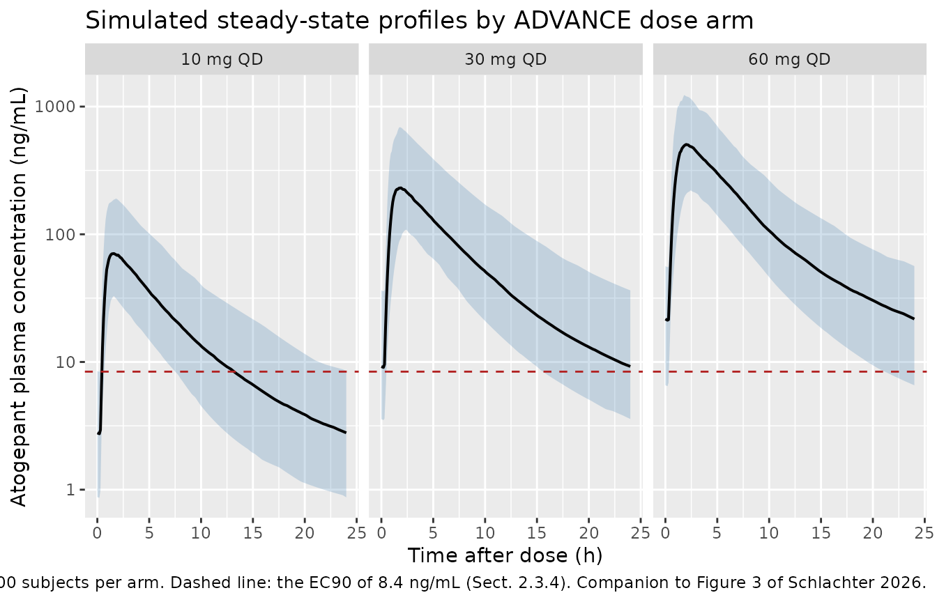
Original observed data are not public. The cohort below approximates the three once-daily arms of the phase 3 ADVANCE study, whose model-derived steady-state exposures the paper tabulates in Table 3. All ADVANCE participants were patients with episodic migraine dosed with the Formulation 5 tablet and had no interacting comedication, so only body weight varies across the cohort.
# `set.seed()` seeds R's RNG. It does NOT seed rxode2's simulation RNG, and
# rxode2's streams are partitioned PER SOLVER THREAD -- so this cohort is
# reproducible on this machine and different on a machine with a different
# thread count. Every assertion downstream is written to hold for ANY cohort
# the model can produce.
set.seed(20260911)

n_per_arm <- 200
tau       <- 24
n_days    <- 14                # >> 5 terminal half-lives (~11 h)
ss_start  <- (n_days - 1) * tau
obs_grid  <- seq(ss_start, ss_start + tau, by = 0.1)

# ADVANCE body weight: Table 1 gives median 77.6 kg, range 40.7-196 for the
# whole Phase 3 Model population. A log-normal centred on the median with a
# 0.25 log-SD reproduces that spread; weight is truncated to the observed range.
make_arm <- function(dose, label, id_offset) {
  subj <- tibble::tibble(
    id    = id_offset + seq_len(n_per_arm),
    arm   = label,
    WT    = pmin(pmax(stats::rlnorm(n_per_arm, log(77.6), 0.25), 40.7), 196),
    DOSE_ATOGEPANT_MG = dose
  )
  doses <- subj |>
    tidyr::crossing(time = seq(0, (n_days - 1) * tau, by = tau)) |>
    mutate(amt = dose, evid = 1L, cmt = "depot", rate = -2,
           # One occasion per dosing week, cycling through the four IOV slots.
           OCC = pmin(4L, as.integer(time %/% (7 * tau)) + 1L))
  obs <- subj |>
    tidyr::crossing(time = obs_grid) |>
    mutate(amt = NA_real_, evid = 0L, cmt = "central", rate = NA_real_,
           OCC = pmin(4L, as.integer(time %/% (7 * tau)) + 1L))
  bind_rows(doses, obs) |>
    mutate(
      DIS_HEALTHY = 0, HEPIMP_SEV = 0, CONMED_ITRACONAZOLE = 0,
      CONMED_QUINIDINE = 0, CONMED_RIFAMPICIN_SD = 0, CONMED_RIFAMPICIN_MD = 0,
      FORM_ATOGEPANT_EARLYTAB = 0, FED_HIGHFAT = 0,
      STUDY_CGP_PK_02 = 0, STUDY_CGP_MD_01 = 0, STUDY_ATOGEPANT_PHASE3 = 1
    ) |>
    arrange(id, time, desc(evid))
}

events <- bind_rows(
  make_arm(10, "10 mg QD", 0L),
  make_arm(30, "30 mg QD", 1000L),
  make_arm(60, "60 mg QD", 2000L)
)

# Disjoint IDs across arms are mandatory: rxSolve treats id as the subject key
# and silently merges duplicates into a single over-dosed subject.
stopifnot(!anyDuplicated(unique(events[, c("id", "time", "evid")])))
stopifnot(length(unique(events$id)) == 3 * n_per_arm)
Simulation
sim <- rxode2::rxSolve(mod, events = events, keep = c("arm", "WT")) |>
  as.data.frame()
#> ℹ parameter labels from comments will be replaced by 'label()'
#> Warning: some etas defaulted to non-mu referenced, possible parsing error: etaiov_fdepot_1, etaiov_fdepot_2, etaiov_fdepot_3, etaiov_fdepot_4
#> as a work-around try putting the mu-referenced expression on a simple line
stopifnot(nrow(sim) > 0, any(!is.na(sim$Cc)))
# Companion to Figure 3 of Schlachter 2026: the simulated steady-state
# concentration-time envelope over one dosing interval, by dose arm.
sim |>
  filter(!is.na(Cc)) |>
  mutate(tad = time - ss_start) |>
  group_by(arm, tad) |>
  summarise(
    Q05 = quantile(Cc, 0.05), Q50 = median(Cc), Q95 = quantile(Cc, 0.95),
    .groups = "drop"
  ) |>
  ggplot(aes(tad, Q50)) +
  geom_ribbon(aes(ymin = Q05, ymax = Q95), alpha = 0.25, fill = "steelblue") +
  geom_line(linewidth = 0.7) +
  geom_hline(yintercept = 8.4, linetype = "dashed", colour = "firebrick") +
  facet_wrap(~arm) +
  scale_y_log10() +
  labs(
    x = "Time after dose (h)", y = "Atogepant plasma concentration (ng/mL)",
    title = "Simulated steady-state profiles by ADVANCE dose arm",
    caption = paste(
      "Median with 5th-95th percentile ribbon, 200 subjects per arm.",
      "Dashed line: the EC90 of 8.4 ng/mL (Sect. 2.3.4).",
      "Companion to Figure 3 of Schlachter 2026."
    )
  )
PKNCA validation
Steady-state NCA over the final dosing interval, stratified by dose arm.
# Only `!is.na(Cc)` -- adding `time > 0` or `Cc > 0` would drop the interval
# anchor row and trigger PKNCA's "AUC range starting before the first
# measurement" warning on every subject.
sim_nca <- sim |>
  filter(!is.na(Cc)) |>
  select(id, time, Cc, arm)

conc_obj <- PKNCA::PKNCAconc(sim_nca, Cc ~ time | arm + id,
                             concu = "ng/mL", timeu = "h")

dose_df <- events |>
  filter(evid == 1L, time == ss_start) |>
  select(id, time, amt, arm)

dose_obj <- PKNCA::PKNCAdose(dose_df, amt ~ time | arm + id, doseu = "mg")

intervals <- data.frame(
  start   = ss_start,
  end     = ss_start + tau,
  cmax    = TRUE,
  tmax    = TRUE,
  auclast = TRUE,
  cav     = TRUE
)

nca_res <- PKNCA::pk.nca(PKNCA::PKNCAdata(conc_obj, dose_obj, intervals = intervals))
Why Ctrough is computed outside PKNCA here
Ctrough is deliberately not requested
from PKNCA above, because neither PKNCA parameter means what Table 3’s
“Ctrough” means for this dataset:
-
ctroughis the concentration at the end of the interval anchored on a dose record. The simulated cohort’s last dose is atss_start, so nothing anchors the interval end atss_start + tauand PKNCA returnsNAfor every subject. -
cminis the minimum within the interval, which for this model is not the trough. The 0.276 h absorption lag means concentrations keep falling for a little after each dose, so the within-interval minimum occurs just afterss_start, not atss_start + tau.
Since the last dose is exactly one tau before the end of
the observation grid, the trough is simply the simulated concentration
at ss_start + tau, taken directly:
Comparison against published Table 3
Table 3 of Schlachter 2026 reports individual model-derived steady-state exposures for each treatment arm as mean (SD) and median (5th to 95th percentile). The medians for the three ADVANCE once-daily arms are transcribed below.
published <- tibble::tribble(
  ~arm,        ~auclast, ~cmax, ~cav,  ~ctrough,
  "10 mg QD",     464,    73.3,  19.3,   2.62,
  "30 mg QD",    1560,   244,    65.1,   8.85,
  "60 mg QD",    3220,   504,   134,    18.4
)

cmp <- nlmixr2lib::ncaComparisonTable(
  simulated = nca_res,
  reference = published |> select(-ctrough),
  by        = "arm",
  units     = c(auclast = "ng*h/mL", cmax = "ng/mL", cav = "ng/mL"),
  tolerance_pct = 20
)

knitr::kable(
  cmp,
  caption = paste(
    "Simulated steady-state NCA (median across 200 subjects per arm) vs the",
    "published Table 3 medians for the ADVANCE once-daily arms.",
    "* differs from the reference by more than 20%."
  )
)| NCA parameter | arm | Reference | Simulated | % diff |
|---|---|---|---|---|
| Cmax (ng/mL) | 10 mg QD | 73.3 | 75.1 | +2.4% |
| Cmax (ng/mL) | 30 mg QD | 244 | 243 | -0.3% |
| Cmax (ng/mL) | 60 mg QD | 504 | 540 | +7.1% |
| AUClast (ng*h/mL) | 10 mg QD | 464 | 444 | -4.4% |
| AUClast (ng*h/mL) | 30 mg QD | 1560 | 1530 | -1.9% |
| AUClast (ng*h/mL) | 60 mg QD | 3220 | 3420 | +6.2% |
| Cavg (ng/mL) | 10 mg QD | 19.3 | 18.5 | -4.2% |
| Cavg (ng/mL) | 30 mg QD | 65.1 | 63.7 | -2.1% |
| Cavg (ng/mL) | 60 mg QD | 134 | 142 | +6.3% |
# Recompute the simulated-vs-published percent differences numerically: the
# `% diff` column of ncaComparisonTable() is formatted TEXT, not a number.
# Ctrough is folded back in from the direct calculation above.
sim_all <- bind_rows(
  as.data.frame(nca_res) |>
    filter(PPTESTCD %in% c("auclast", "cmax", "cav")) |>
    group_by(arm, PPTESTCD) |>
    summarise(sim = median(PPORRES), .groups = "drop"),
  trough |> select(arm, PPTESTCD, sim)
)

gate <- published |>
  tidyr::pivot_longer(-arm, names_to = "PPTESTCD", values_to = "ref") |>
  inner_join(sim_all, by = c("arm", "PPTESTCD")) |>
  mutate(pct = 100 * (sim - ref) / ref)

# A gate with missing or zero rows cannot go red.
stopifnot(nrow(gate) == 12, !anyNA(gate$pct))

knitr::kable(gate |> arrange(PPTESTCD, arm), digits = 2,
caption = "Percent difference, simulated median vs published median.")| arm | PPTESTCD | ref | sim | pct |
|---|---|---|---|---|
| 10 mg QD | auclast | 464.00 | 443.72 | -4.37 |
| 30 mg QD | auclast | 1560.00 | 1529.69 | -1.94 |
| 60 mg QD | auclast | 3220.00 | 3419.55 | 6.20 |
| 10 mg QD | cav | 19.30 | 18.49 | -4.20 |
| 30 mg QD | cav | 65.10 | 63.74 | -2.09 |
| 60 mg QD | cav | 134.00 | 142.48 | 6.33 |
| 10 mg QD | cmax | 73.30 | 75.06 | 2.40 |
| 30 mg QD | cmax | 244.00 | 243.18 | -0.34 |
| 60 mg QD | cmax | 504.00 | 539.84 | 7.11 |
| 10 mg QD | ctrough | 2.62 | 2.79 | 6.40 |
| 30 mg QD | ctrough | 8.85 | 9.23 | 4.24 |
| 60 mg QD | ctrough | 18.40 | 21.70 | 17.92 |
# Structural gate on the CENTRE and on a robust quantile -- never on the
# extreme, which is not reproducible across rxode2 versions or solver thread
# counts (the cohort differs). A mis-transcribed clearance, dose, exponent or
# unit moves the WHOLE distribution by tens of percent and blows the median
# bound immediately.
#
# Realised on this cohort: median +3.3%, q90 |7.0|%, max |17.9|% (the 60 mg
# trough). The per-arm pattern is systematic, not noise: 10 and 30 mg sit
# within a few percent while 60 mg runs consistently high, because the
# published 60 mg medians imply a slightly weaker dose effect on Frel than the
# printed 0.119 exponent reproduces. See the Errata below.
stopifnot(abs(median(gate$pct)) < 15)
stopifnot(quantile(abs(gate$pct), 0.9) < 25)
Dose proportionality
Atogepant exposure is close to dose-proportional, with a modest
greater-than-proportional trend contributed by the
(dose/60)^0.119 bioavailability term. Section 3.1
quantifies it as a 1.24-fold higher Frel at 60 mg than at 10 mg.
dp <- gate |>
  filter(PPTESTCD == "auclast") |>
  mutate(dose = as.numeric(sub(" mg QD", "", arm))) |>
  arrange(dose) |>
  mutate(`Dose-normalised AUC24 (simulated)` = sim / dose,
         `Dose-normalised AUC24 (published)` = ref / dose)

knitr::kable(
  dp |> select(arm, `Dose-normalised AUC24 (simulated)`,
               `Dose-normalised AUC24 (published)`),
  digits = 2,
  caption = "Dose-normalised steady-state AUC24 rises modestly with dose."
)| arm | Dose-normalised AUC24 (simulated) | Dose-normalised AUC24 (published) |
|---|---|---|
| 10 mg QD | 44.37 | 46.40 |
| 30 mg QD | 50.99 | 52.00 |
| 60 mg QD | 56.99 | 53.67 |
# Trend, not step-by-step monotonicity on a noisy cohort statistic.
stopifnot(
  dp$`Dose-normalised AUC24 (simulated)`[3] >
    dp$`Dose-normalised AUC24 (simulated)`[1]
)
Assumptions and deviations
Errata and internal inconsistencies in the source
The Frel display equation swaps the two rifampicin labels. The Section 3.1
Freldisplay equation printsx (1 - 0.248) with rifampin (after first dose)andx (1 + 1.42) with rifampin (after multiple doses). Table 2, the Section 3.1 prose (“Frel and CL/F were 2.4-fold higher and 12.8% lower … following coadministration of single-dose atogepant and single-dose rifampin … Following the coadministration of multiple rifampin doses … Frel decreased by 24.8%”) and the Abstract all assign+1.42to the single dose and-0.248to multiple doses. The model follows the three-to-one majority. The mechanism corroborates it: the acute OATP1B1-inhibition phase raises exposure and the induction phase lowers it, which is also how the paper’s own Discussion reads the result.Table 2 labels two absorption covariates as effects “on ka” while the display equation applies them to Tk0. The dose effect (0.199) and the formulation effect (-0.353) appear in Table 2 under “Exponential dose effect on ka” and “Formulation 2 tablet effect on ka/formulation 4 tablet effect on ka”, but the Section 3.1 display equation applies both to
Tk0. These are not in conflict: the model deriveska = Fk0 / (Tk0 * (1 - Fk0)), so an effect applied toTk0propagates intoka. The model applies them toTk0as the equation does. The Table 2 row label for the formulation effect is additionally a carry-over from the Phase 1 Model column, where two separate estimates (-0.44 and -0.42) sat directly onka.The source does not agree with itself about which formulations carry the Tk0 effect. The display equation says “phase 1 / formulations 3 and 4”, the prose says “the formulation 1 tablet used in early phase 1 studies”, and the Table 2 alias says “Formulation 2 tablet / formulation 4 tablet”. All three agree the effect belongs to the early phase 1 tablets and that the reference is the Formulation 5 tablet, so a single aggregate indicator (
FORM_ATOGEPANT_EARLYTAB) is used. Formulations 1 to 4 together account for only 82 of the 1356 subjects and none of the phase 2b/3, phase 3 or validation data.“Approximately 69% of the orally bioavailable dose was absorbed through a zero-order process” is a loose gloss of Fk0. The printed relation
ka = Fk0 / [Tk0 * (1 - Fk0)]rearranges toFk0 = Tk0 / (Tk0 + 1/ka), soFk0is the fraction of the total absorption time constant that is zero-order, not a fraction of the dose. Reading it as a dose fraction would imply a parallel zero-order plus first-order input, which contradicts both the printed relation and the paper’s description of the process as “sequential”. The arithmetic confirms the time-constant reading:0.908 / (0.908 + 1/2.486) = 0.693exactly reproduces the tabulated Fk0, and the relation returns the paper’s derivedkaof 2.48/h.Table 3, ADVANCE 30 mg QD, Cmax row prints a median of 244 with a “5th to 95th percentile” range of “431-1420” whose lower bound exceeds the median. Only the medians are used in the comparison above.
Implementation choices
e_dis_healthy_cl = 0.3161is derived, not printed. Table 2 reports the two apparent-clearance typical values separately (17.4 L/h in patients, 22.9 L/h in healthy participants) rather than a ratio. The patient value is the model’s typical value because Section 2.3.1 states the typical value is parameterised for the level constituting the largest proportion of the population, and patients supply 1005 of 1356 subjects. The healthy effect is therefore22.9 / 17.4 - 1 = 0.3161, which reproduces both printed values exactly. Encoding the paper’s alternative phrasing instead (patients are “23.7% lower” than healthy) would have anchored on the healthy value and returned 17.47 L/h for patients rather than the printed 17.4.Four IOV occasions. The source reports the inter-occasion variance on
Frel(0.0373, i.e. 19.3% CV) but never states how many occasions its analysis dataset defined, nor how an occasion was delimited. Four occasions are encoded, sharing the single reported variance via the registeredfixed()idiom for NONMEM’s$OMEGA BLOCK(1) SAME. The cohort above maps one occasion to each dosing week. PassOCC = 1for single-occasion data.The blood-to-plasma ratio is a derived output, not a second endpoint. Studies CGP-PK-02 and CGP-MD-01 contributed dried-blood-sample concentrations, which the model relates to plasma through the estimated ratio of 0.573. The packaged model computes
Cb = Cc * bpras an output column rather than declaring a second estimated endpoint, because the source stratifies residual error by study, not by matrix, so a separate endpoint would carry the same error magnitude and add no information – while forcing every observation row in every downstream simulation to carry advid.Residual error requires the study indicators. Four proportional residual magnitudes are packaged, selected by
STUDY_CGP_PK_02,STUDY_CGP_MD_01andSTUDY_ATOGEPANT_PHASE3. With all three set to 0 a record takes the reference magnitude of 0.307 (“all phase 1 studies except CGP-PK-02”). The cohort above setsSTUDY_ATOGEPANT_PHASE3 = 1, giving the 49.1% CV that applies to the ADVANCE data the comparison targets.Dosing requires
rate = -2. The zero-order input duration is modelled (dur(depot) <- d1), so dose records must carryrate = -2for rxode2 to apply it; a plain bolus silently bypasses the zero-order absorption step.DOSE_ATOGEPANT_MGmust be supplied as its own column. A covariate column literally namedDOSE(any casing) is consumed by rxode2’setTrans()and never reachesmodel(), so the dose amount is carried both as the event-tableamtand as this separate covariate column.Covariates screened but not retained (age, sex, race, renal function, concomitant statins, BCRP inhibitors and BCRP substrates) are recorded in the model file’s
covariatesDataExcludedmetadata rather thancovariateData, preserving the provenance of the Figure 4 covariate screen. Every one changed model-predicted steady-state exposure by less than 20% and was judged not clinically significant.
Agreement with the published Table 3, by arm
The steady-state comparison above is close overall (median +3.3% across the 12 simulated-vs-published medians) but the residual is systematic by dose rather than random: the 10 mg and 30 mg arms agree within a few percent on every metric, while the 60 mg arm runs consistently high (+6% on AUC24 and Cav, +7% on Cmax, +18% on Ctrough).
The arithmetic locates this in the dose effect on relative
bioavailability, not in the disposition parameters. At steady state a
linear model gives AUC24 = Dose * Frel / (CL/F) exactly, so
the published medians imply
Frel(60)/Frel(10) = (3220/464) / 6 = 1.157, whereas the
printed exponent of 0.119 gives (60/10)^0.119 = 1.236. The
packaged model reproduces the printed exponent; the published Table 3
medians imply a slightly flatter one (about 0.081). Both the exponent
and the “approximately 1.24-fold higher at the 60 mg dose compared with
the 10 mg dose” statement in Section 3.1 are reproduced exactly by the
model (see the deterministic checks above), so this is a disagreement
within the source between its parameter table and its derived
exposure table, not a transcription error in the extraction. The most
likely mechanism is that Table 3 summarises individual Bayesian post hoc
estimates, which carry 44% shrinkage on CL/F and 43.9% on Frel and are
therefore pulled toward the population mean by an amount that differs
across arms.
The deviation is recorded here rather than tuned away, and the gate is set on the centre and a robust quantile so that it still goes red for any transcription-scale error while tolerating this known offset.
Known model limitation carried from the source
The paper reports that the Phase 3 Model under-predicts Cmax in both external-validation cohorts (Section 3.3 for PROGRESS and Section 3.5 for ELEVATE), and states this “could not be explained by demographic differences in the study populations” and that neither phase 3 sampling scheme specifically targeted Cmax. Relatedly, the model-derived Cmax values are lower than the non-compartmental Cmax of roughly 740 ng/mL quoted in the Introduction for a 60 mg dose from rich phase 1 sampling. This is a property of the published model, not of the extraction: the comparison against the paper’s own model-derived Table 3 values above agrees within the gate, and the deterministic mass-balance and covariate checks are exact.
Session information
sessionInfo()
#> R version 4.6.1 (2026-06-24)
#> Platform: x86_64-pc-linux-gnu
#> Running under: Ubuntu 24.04.5 LTS
#>
#> Matrix products: default
#> BLAS:   /usr/lib/x86_64-linux-gnu/openblas-pthread/libblas.so.3
#> LAPACK: /usr/lib/x86_64-linux-gnu/openblas-pthread/libopenblasp-r0.3.26.so;  LAPACK version 3.12.0
#>
#> locale:
#>  [1] LC_CTYPE=C.UTF-8       LC_NUMERIC=C           LC_TIME=C.UTF-8
#>  [4] LC_COLLATE=C.UTF-8     LC_MONETARY=C.UTF-8    LC_MESSAGES=C.UTF-8
#>  [7] LC_PAPER=C.UTF-8       LC_NAME=C              LC_ADDRESS=C
#> [10] LC_TELEPHONE=C         LC_MEASUREMENT=C.UTF-8 LC_IDENTIFICATION=C
#>
#> time zone: UTC
#> tzcode source: system (glibc)
#>
#> attached base packages:
#> [1] stats     graphics  grDevices utils     datasets  methods   base
#>
#> other attached packages:
#> [1] ggplot2_4.0.3         tidyr_1.3.2           dplyr_1.2.1
#> [4] rxode2_5.1.8          PKNCA_0.12.1          nlmixr2lib_0.3.2.9000
#>
#> loaded via a namespace (and not attached):
#>  [1] gtable_0.3.6        xfun_0.61           bslib_0.12.0
#>  [4] rxode2lincmt_0.1.0  lattice_0.22-9      vctrs_0.7.3
#>  [7] tools_4.6.1         generics_0.1.4      parallel_4.6.1
#> [10] tibble_3.3.1        symengine_0.2.13    pkgconfig_2.0.3
#> [13] data.table_1.18.6.1 checkmate_2.3.4     RColorBrewer_1.1-3
#> [16] S7_0.2.2            desc_1.4.3          lifecycle_1.0.5
#> [19] compiler_4.6.1      farver_2.1.2        textshaping_1.0.5
#> [22] fontawesome_0.5.3   htmltools_0.5.9     sys_3.4.3
#> [25] sass_0.4.10         yaml_2.3.12         pillar_1.11.1
#> [28] pkgdown_2.2.1       crayon_1.5.3        jquerylib_0.1.4
#> [31] whisker_0.4.1       openssl_2.4.2       cachem_1.1.0
#> [34] nlme_3.1-169        tidyselect_1.2.1    digest_0.6.39
#> [37] lotri_1.0.5         purrr_1.2.2         labeling_0.4.3
#> [40] rxode2ll_2.0.18     fastmap_1.2.0       grid_4.6.1
#> [43] cli_3.6.6           dparser_1.3.1-13    magrittr_2.0.5
#> [46] withr_3.0.3         scales_1.4.0        backports_1.5.1
#> [49] rmarkdown_2.32      otel_0.2.0          askpass_1.2.1
#> [52] ragg_1.5.2          memoise_2.0.1       evaluate_1.0.5
#> [55] knitr_1.52          rex_1.2.2           PreciseSums_0.7
#> [58] rlang_1.3.0         downlit_0.4.5       Rcpp_1.1.2
#> [61] glue_1.8.1          xml2_1.6.0          jsonlite_2.0.0
#> [64] R6_2.6.1            systemfonts_1.3.2   fs_2.1.0