Rifampicin (Vinnard 2017)
Source:vignettes/articles/Vinnard_2017_rifampicin.Rmd
Vinnard_2017_rifampicin.RmdModel and source
- Citation: Vinnard C, Ravimohan S, Tamuhla N, Pasipanodya J, Srivastava S, Modongo C, Zetola NM, Weissman D, Gumbo T, Bisson GP. (2017). Markers of gut dysfunction do not explain low rifampicin bioavailability in HIV-associated TB. J Antimicrob Chemother 72(7):2020-2027. doi:10.1093/jac/dkx111.
- Description: One-compartment population PK model for oral rifampicin in HIV/TB patients in Botswana (Vinnard 2017), with a Savic 2007 analytical transit-compartment absorption chain feeding a virtual depot, oral bioavailability fixed at 1, between-subject variability on CL, F, MTT, and the (non-integer) number of transit compartments NN, and inter-occasion variability on F across two sampling visits (pre-ART vs after approximately 4 weeks of ART).
- Article: J Antimicrob Chemother 72(7):2020-2027
The Vinnard 2017 cohort recruited HIV-infected adults newly diagnosed with pulmonary TB in Gaborone, Botswana, and characterised rifampicin pharmacokinetics across two visits: the first 5-28 days after starting standard first-line antitubercular therapy (pre-ART) and the second approximately 4 weeks after initiating efavirenz-based ART. The primary research question was whether plasma markers of gut damage (I-FABP), microbial translocation (sCD14), or systemic immune activation (%CD38+DR+CD8+, IL-6) explained variability in rifampicin bioavailability F; the paper concluded that none of these covariates significantly reduced the objective function value (Table 2), so the final structural PK model in Table 1 carries no covariate effects.
Population
40 HIV-infected adults completed the first pharmacokinetic visit; 24 of those returned for the second visit after approximately 4 weeks of ART. Median age was 32 years (IQR 27-43) and median CD4 T-cell count was 238 cells/uL (IQR 105-339). Patients were dosed once daily according to WHO weight-based rifampicin bands: 300 mg (n = 1), 450 mg (n = 19), 600 mg (n = 17), or 750 mg (n = 3) – corresponding to 7.9-12.5 mg/kg, median 9.7 mg/kg. All patients received tenofovir + emtricitabine + efavirenz at the second visit.
The same population information is available programmatically via
rxode2::rxode(readModelDb("Vinnard_2017_rifampicin"))$population.
Source trace
The per-parameter origin is recorded as an in-file comment next to
each ini() entry in
inst/modeldb/specificDrugs/Vinnard_2017_rifampicin.R. The
table below collects them in one place for review.
| Equation / parameter | Value | Source location |
|---|---|---|
| Oral apparent clearance CL/F | 16.36 L/h | Vinnard 2017 Table 1, row “oral apparent clearance (CL/F) (L/h)” |
| Oral apparent volume V/F | 52.90 L | Vinnard 2017 Table 1, row “oral apparent volume of distribution (V/F) (L)” |
| Mean transit time MTT | 0.97 h | Vinnard 2017 Table 1, row “mean transit time within compartments (h)” |
| Number of transit cmts NN | 4.36 | Vinnard 2017 Table 1, row “number of absorption transit compartments” |
| Oral bioavailability F | 1 (fixed) | Vinnard 2017 Table 1, row “oral bioavailability (F)” |
| BSV CL/F | 32.4% CV | Vinnard 2017 Table 1, row “between-subject variability of clearance (%)” |
| BSV F | 21.1% CV | Vinnard 2017 Table 1, row “between-subject variability of bioavailability (%)” |
| BSV NN | 85.8% CV | Vinnard 2017 Table 1, row “between-subject variability of the number of transit compartments (%)” |
| BSV MTT | 55.7% CV | Vinnard 2017 Table 1, row “between-subject variability of the mean transit time (%)” |
| IOV F | 9.2% CV | Vinnard 2017 Table 1, row “inter-occasional variability in bioavailability (%)” |
| Proportional residual error | 0.37 | Vinnard 2017 Table 1, row “proportional error (% CV)” |
| Additive residual error | 0.16 mg/L | Vinnard 2017 Table 1, row “additive error (SD, mg/L)” |
| Absorption: Savic 2007 transit chain | n/a | Vinnard 2017 Methods “Non-linear mixed-effects modelling of pharmacokinetic data” (transit compartment model citing Savic 2007 ref. 34) |
| 1-compartment, first-order elimination | n/a | Vinnard 2017 Results paragraph 4 (“best explained by a one-compartment model with first-order elimination”) |
| No structural covariates | n/a | Vinnard 2017 Table 2 (no covariate reduced OFV significantly) |
Virtual cohort
The original individual-level data are not publicly available. The figures below build a virtual cohort matching the published dose distribution (Table footnote and Results paragraph 1: 300 mg n = 1, 450 mg n = 19, 600 mg n = 17, 750 mg n = 3).
set.seed(20260521)

dose_counts <- tibble::tibble(
  amt_mg = c(300, 450, 600, 750),
  n      = c(1L, 19L, 17L, 3L)
)
n_total <- sum(dose_counts$n)

make_cohort <- function(dose_counts, occ, sample_times, id_offset = 0L) {
  id_vec <- seq_len(sum(dose_counts$n))
  amt_vec <- rep(dose_counts$amt_mg, dose_counts$n)
  dose_rows <- tibble::tibble(
    id   = id_offset + id_vec,
    time = 0,
    amt  = amt_vec,
    evid = 1L,
    cmt  = "depot",
    OCC  = occ,
    treatment = sprintf("%d mg", amt_vec)
  )
  obs_rows <- tidyr::expand_grid(
    id = id_offset + id_vec,
    time = sample_times
  ) |>
    dplyr::left_join(
      tibble::tibble(id = id_offset + id_vec,
                     amt_mg = amt_vec),
      by = "id"
    ) |>
    dplyr::mutate(
      amt = 0,
      evid = 0L,
      cmt = "central",
      OCC = occ,
      treatment = sprintf("%d mg", amt_mg)
    ) |>
    dplyr::select(id, time, amt, evid, cmt, OCC, treatment)
  dplyr::bind_rows(dose_rows, obs_rows) |>
    dplyr::arrange(id, time, dplyr::desc(evid))
}

# Pre-ART occasion (OCC = 1) sampled densely for VPC plots.
events <- make_cohort(
  dose_counts  = dose_counts,
  occ          = 1,
  sample_times = seq(0, 24, by = 0.25),
  id_offset    = 0L
)
stopifnot(!anyDuplicated(unique(events[, c("id", "time", "evid")])))
Simulation
mod <- rxode2::rxode(readModelDb("Vinnard_2017_rifampicin"))
#> ℹ parameter labels from comments will be replaced by 'label()'
#> Warning: some etas defaulted to non-mu referenced, possible parsing error: etaiov_fdepot_1, etaiov_fdepot_2
#> as a work-around try putting the mu-referenced expression on a simple line

# Stochastic VPC-style simulation with full between-subject and inter-occasion
# variability.
set.seed(20260521)
sim <- rxode2::rxSolve(
  mod,
  events = events,
  keep = c("treatment", "OCC")
) |>
  as.data.frame()
For deterministic typical-value replication (no random effects),
zeroRe() gives the population mean prediction:
mod_typical <- rxode2::zeroRe(mod)
#> Warning: some etas defaulted to non-mu referenced, possible parsing error: etaiov_fdepot_1, etaiov_fdepot_2
#> as a work-around try putting the mu-referenced expression on a simple line
sim_typical <- rxode2::rxSolve(
  mod_typical,
  events = events,
  keep = c("treatment", "OCC")
) |>
  as.data.frame()
#> ℹ omega/sigma items treated as zero: 'etalcl', 'etalfdepot', 'etalnn', 'etalmtt', 'etaiov_fdepot_1', 'etaiov_fdepot_2'
#> Warning: multi-subject simulation without without 'omega'
Replicate published figures
Figure 1 - Mean rifampicin concentration vs time
Vinnard 2017 Figure 1 plots mean rifampicin concentration-vs-time curves grouped by the SLCO1B1 rs11045819 variant allele genotype. The packaged model does not encode SLCO1B1 genotype (the paper found a significant AUC difference by NCA but could not formally evaluate it in the population model because of the highly skewed allele distribution; Discussion paragraph 4 / Limitations). The corresponding mean concentration curve is shown below for the full simulated cohort, faceted by dose band.
sim_typical |>
  dplyr::filter(time > 0) |>
  ggplot(aes(time, Cc)) +
  geom_line() +
  facet_wrap(~ treatment) +
  labs(
    x = "Time post-dose (h)",
    y = "Rifampicin Cc (mg/L)",
    title = "Typical-value rifampicin concentration vs time by dose band",
    caption = "Replicates the form of Figure 1 of Vinnard 2017 (typical value)."
  )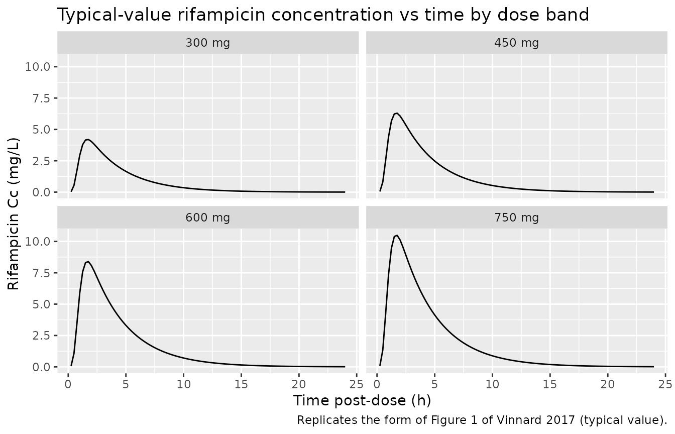
Replicates the structural mean-concentration form of Figure 1 of Vinnard 2017 (typical-value time course; SLCO1B1 covariate omitted because the population model does not carry it).
Figure 3 - Cmax and AUC0-24 distributions
cmax_per_id <- sim |>
  dplyr::group_by(id, treatment) |>
  dplyr::summarise(
    Cmax = max(Cc, na.rm = TRUE),
    .groups = "drop"
  )

ggplot(cmax_per_id, aes(treatment, Cmax)) +
  geom_boxplot() +
  geom_jitter(width = 0.15, alpha = 0.6) +
  labs(
    x = "Rifampicin dose band",
    y = "Cmax (mg/L)",
    title = "Simulated Cmax by dose band (pre-ART, OCC = 1)",
    caption = "Replicates the spread of Vinnard 2017 Figure 3a (Cmax)."
  )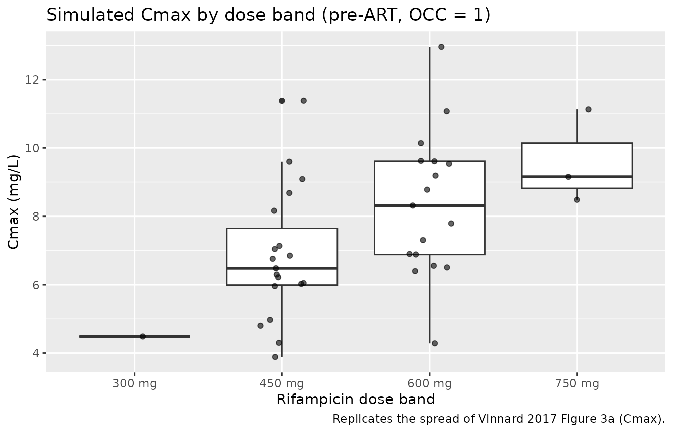
Distributions of simulated Cmax and AUC0-24 across 40 subjects on the published dose band distribution; pre-ART occasion (OCC = 1).
PKNCA validation
PKNCA computes Cmax, Tmax, AUC0-24 (matching the paper’s reported AUC0-8 and AUC0-24 endpoints), and half-life. The treatment grouping is the dose band.
sim_nca <- sim |>
  dplyr::filter(!is.na(Cc)) |>
  dplyr::select(id, time, Cc, treatment) |>
  dplyr::distinct(id, time, .keep_all = TRUE)

dose_df <- events |>
  dplyr::filter(evid == 1) |>
  dplyr::select(id, time, amt, treatment)

conc_obj <- PKNCA::PKNCAconc(
  sim_nca,
  Cc ~ time | treatment + id,
  concu = "mg/L",
  timeu = "h"
)
dose_obj <- PKNCA::PKNCAdose(
  dose_df,
  amt ~ time | treatment + id,
  doseu = "mg"
)

intervals <- data.frame(
  start       = c(0, 0),
  end         = c(8, 24),
  cmax        = c(TRUE, TRUE),
  tmax        = c(TRUE, TRUE),
  auclast     = c(TRUE, TRUE),
  half.life   = c(FALSE, TRUE)
)

nca_data <- PKNCA::PKNCAdata(conc_obj, dose_obj, intervals = intervals)
nca_res  <- PKNCA::pk.nca(nca_data)

nca_tbl <- as.data.frame(nca_res$result)
knitr::kable(
  head(nca_tbl, 12),
  caption = "First 12 rows of the per-subject PKNCA result table."
)| treatment | id | start | end | PPTESTCD | PPORRES | exclude | PPORRESU |
|---|---|---|---|---|---|---|---|
| 300 mg | 1 | 0 | 8 | auclast | 20.7683115 | NA | h*mg/L |
| 300 mg | 1 | 0 | 8 | cmax | 4.4855222 | NA | mg/L |
| 300 mg | 1 | 0 | 8 | tmax | 2.7500000 | NA | h |
| 300 mg | 1 | 0 | 24 | auclast | 26.2911944 | NA | h*mg/L |
| 300 mg | 1 | 0 | 24 | cmax | 4.4855222 | NA | mg/L |
| 300 mg | 1 | 0 | 24 | tmax | 2.7500000 | NA | h |
| 300 mg | 1 | 0 | 24 | tlast | 24.0000000 | NA | h |
| 300 mg | 1 | 0 | 24 | lambda.z | 0.2477855 | NA | 1/h |
| 300 mg | 1 | 0 | 24 | r.squared | 0.9999424 | NA | unitless |
| 300 mg | 1 | 0 | 24 | adj.r.squared | 0.9999417 | NA | unitless |
| 300 mg | 1 | 0 | 24 | lambda.z.time.first | 3.0000000 | NA | h |
| 300 mg | 1 | 0 | 24 | lambda.z.time.last | 24.0000000 | NA | h |
Comparison against published NCA medians
Vinnard 2017 Results paragraph 7 reports observed cohort-level NCA medians at visit 1 (pre-ART): Cmax 7.4 mg/L (range 2.56-11.61), AUC0-24 34.4 mg*h/L (range 8.2-80.2). The simulated cohort below mixes the published dose-band distribution (300, 450, 600, 750 mg with n = 1, 19, 17, 3) so the simulated medians are directly comparable to the observed cohort-level medians.
nca_summary <- nca_tbl |>
  dplyr::filter(PPTESTCD %in% c("cmax", "auclast")) |>
  dplyr::group_by(PPTESTCD, start, end) |>
  dplyr::summarise(
    median = median(PPORRES, na.rm = TRUE),
    q05    = quantile(PPORRES, 0.05, na.rm = TRUE),
    q95    = quantile(PPORRES, 0.95, na.rm = TRUE),
    .groups = "drop"
  )

published <- tibble::tibble(
  endpoint = c("Cmax (mg/L)", "AUC0-24 (mg*h/L)"),
  observed_median = c(7.4, 34.4),
  observed_range  = c("2.56-11.61", "8.2-80.2")
)

compare <- nca_summary |>
  dplyr::mutate(
    endpoint = dplyr::case_when(
      PPTESTCD == "cmax"    ~ "Cmax (mg/L)",
      PPTESTCD == "auclast" & end == 24 ~ "AUC0-24 (mg*h/L)",
      PPTESTCD == "auclast" & end == 8  ~ "AUC0-8 (mg*h/L)",
      TRUE ~ PPTESTCD
    )
  ) |>
  dplyr::filter(endpoint %in% c("Cmax (mg/L)", "AUC0-24 (mg*h/L)")) |>
  dplyr::left_join(published, by = "endpoint") |>
  dplyr::transmute(
    endpoint,
    simulated_median = round(median, 2),
    simulated_5_95   = sprintf("%.2f - %.2f", q05, q95),
    observed_median,
    observed_range
  )

knitr::kable(compare, caption = "Simulated vs Vinnard 2017 observed pre-ART NCA medians.")| endpoint | simulated_median | simulated_5_95 | observed_median | observed_range |
|---|---|---|---|---|
| AUC0-24 (mg*h/L) | 31.94 | 19.00 - 53.25 | 34.4 | 8.2-80.2 |
| Cmax (mg/L) | 7.09 | 4.30 - 11.15 | 7.4 | 2.56-11.61 |
| Cmax (mg/L) | 7.09 | 4.30 - 11.15 | 7.4 | 2.56-11.61 |
Assumptions and deviations
No covariates carried into simulation. The paper evaluated I-FABP, sCD14, %CD38+DR+CD8+, IL-6, CD4 T-cell count, and HIV viral load on F and none significantly reduced the OFV (Table 2). The packaged model therefore carries no covariate effects on the structural PK parameters. Users simulating sub-populations stratified by these markers will get identical typical-value predictions; only between-subject variability scatter them.
SLCO1B1 genotype not encoded. Figure 1 of the source paper stratifies mean concentration curves by the SLCO1B1 rs11045819 variant allele (Discussion paragraph 4), but the population model in Table 1 does not include genotype because of the highly skewed allele distribution in the cohort (paper Limitations paragraph 2: “The highly skewed distribution of SLCO1B1 genotypes in the study population prevented formal evaluation of genotype effects in the population pharmacokinetic model.”). The simulated Figure 1 above therefore reproduces only the cohort-average curve, not the genotype-stratified curves.
No explicit first-order absorption rate ka. The paper reports only the transit-compartment parameters MTT and NN (Table 1) and cites Savic 2007 for the analytical input-rate form. Following the established Wilkins_2008_rifampicin / Tikiso_2021_abacavir / vanderWalt_2013_dapagliflozin pattern in nlmixr2lib, the implementation uses rxode2’s built-in
transit(NN, MTT, fdepot)to deliver the Savic-2007 gamma-PDF input rate into the depot, then a virtual fast absorption rateka = 60/h (depot half-life approximately 0.012 h, an order of magnitude faster than KTR = (NN + 1)/MTT approximately 5.5 /h) collapses the depot’s exponential tail so the central-compartment input rate effectively tracks the transit() gamma-PDF directly. This preserves the Savic-2007 absorption shape without introducing a phantom absorption phase.Inter-occasion variability multiplexed by
OCC. The 9.2% CV IOV on F reported in Table 1 spans the two pharmacokinetic visits (pre-ART and approximately 4 weeks after ART). Simulation users must supply anOCCcolumn on each event record with values 1 (pre-ART) or 2 (post-ART); other integer values yield zero IOV contribution. The packaged variance is shared across both occasions, matching the source’s single IOV variance estimate (no NONMEM-styleBLOCK(1) SAMEshortcut exists in nlmixr2, so the second occasion’s eta is declared withfix()equal to the first).Volume V/F carries no BSV. Vinnard 2017 Table 1 reports between-subject variability on CL, F, NN, and MTT only; V/F has no BSV row. The packaged model therefore has no
etalvcterm.Weight not used in dose normalisation. Patients in the trial received weight-band-based doses (WHO 2010 guidelines), but the structural model does not include allometric scaling on CL/V. Simulation users must supply explicit
amtvalues per subject; mg/kg dose normalisation is done outside the model.Auto-induction not separately estimated. Limitations paragraph 1 notes that the visit-1 sampling window (5-28 days post-treatment-initiation) and the visit-2 timing prevented an independent estimate of baseline vs steady-state clearance after rifampicin auto-induction. The packaged parameters therefore represent the post-induction steady-state CL/F. For models requiring an explicit autoinduction time-course, see
Svensson_2016_rifampicin(enzyme-pool turnover) orSvensson_2018_rifampicin(DDMORE bundle).