Empagliflozin renal glucose threshold in type 1 vs type 2 diabetes (Mondick 2018)
Source:vignettes/articles/Mondick_2018_empagliflozin.Rmd
Mondick_2018_empagliflozin.RmdModel and source
Mondick 2018 contributes two model files, one per patient population, both pointing at this article:
-
Mondick_2018_empagliflozin_t1dm– the paper’s own type 1 diabetes (T1DM) fit. -
Mondick_2018_empagliflozin_t2dm– the type 2 diabetes (T2DM) parameter set that the paper reproduces in Supplementary Table 2 and uses for its T1DM-vs-T2DM comparison (Figures 4 and 5).
mod_t1dm <- readModelDb("Mondick_2018_empagliflozin_t1dm")
mod_t2dm <- readModelDb("Mondick_2018_empagliflozin_t2dm")

ui_t1dm <- rxode2::rxode(mod_t1dm)
#> ℹ parameter labels from comments will be replaced by 'label()'
ui_t2dm <- rxode2::rxode(mod_t2dm)
#> ℹ parameter labels from comments will be replaced by 'label()'- Citation: Mondick J, Riggs M, Kaspers S, Soleymanlou N, Marquard J, Nock V. Population pharmacokinetic-pharmacodynamic analysis to characterize the effect of empagliflozin on renal glucose threshold in patients with type 1 diabetes mellitus. J Clin Pharmacol. 2018;58(5):640-649. doi:10.1002/jcph.1051. The PD structure follows the type 2 diabetes model of Mondick J, Riggs M, Sasaki T, Sarashina A, Broedl UC, Retlich S. Diabetes Obes Metab. 2016;18:241-248; see modellib(‘Mondick_2018_empagliflozin_t2dm’) for that population’s parameter set as reproduced in Mondick 2018 Supplementary Table 2.
- Article: https://doi.org/10.1002/jcph.1051
Population
The T1DM model was developed from EASE-1 (NCT01969747), a randomized, placebo-controlled, parallel-group phase 2 study of once-daily oral empagliflozin as an adjunct to insulin, run at one German and one Austrian centre between 25 November 2013 and 20 April 2014. Seventy-five patients were randomized 1:1:1:1 to placebo (n = 19), empagliflozin 2.5 mg (n = 19), 10 mg (n = 19) or 25 mg (n = 18) for 28 days.
At baseline the cohort had mean (SD) age 41.0 (10.9) years, body mass index 25.6 (3.69) kg/m^2, weight 79.3 (14.3) kg and eGFR 102 (13.8) mL/(min * 1.73 m^2); 53/75 (71%) were male. The population PK data set held 1814 empagliflozin concentrations and the PD data set 900 urinary glucose excretion records (Mondick 2018, Results, “Analysis Population”). The reference patient for the covariate model is a 42-year-old male.
The T2DM parameter set was estimated in Mondick 2016 (Diabetes Obes Metab 18:241-248) from four phase 1 and phase 2 empagliflozin trials spanning 1-100 mg, with one further study used for model evaluation; its reference patient is a 58-year-old male. Mondick 2018 does not restate that cohort’s size or demographics.
str(ui_t1dm$population)
#> List of 13
#>  $ species       : chr "human"
#>  $ n_subjects    : num 75
#>  $ n_studies     : num 1
#>  $ age_range     : chr "20-60 years"
#>  $ age_median    : chr "41.0 years (mean; SD 10.9). Reference patient 42 years"
#>  $ weight_median : chr "79.3 kg (mean; SD 14.3)"
#>  $ bmi_median    : chr "25.6 kg/m^2 (mean; SD 3.69)"
#>  $ sex_female_pct: num 29.3
#>  $ renal_function: chr "eGFR mean 102 mL/min/1.73 m^2 (SD 13.8)"
#>  $ disease_state : chr "type 1 diabetes mellitus, on background insulin"
#>  $ dose_range    : chr "placebo, or empagliflozin 2.5, 10 or 25 mg orally once daily for 28 days, as adjunct to insulin"
#>  $ regions       : chr "Germany, Austria"
#>  $ notes         : chr "EASE-1 (NCT01969747), a randomized, placebo-controlled, parallel-group phase 2 study run at one German and one "| __truncated__
Model structure
The PK and PD layers were fitted sequentially: the PK model by FOCE with eta-epsilon interaction, then the PD model by SAEM with the individual empirical Bayes PK estimates supplied as input.
Empagliflozin disposition is a two-compartment model with sequential zero- then first-order absorption and an absorption lag time. Body size enters only through BMI, as a power term on CL/F, Vc/F, Q/F and Vp/F referenced to 25 kg/m^2.
The PD layer is mechanistic. Urinary glucose excretion is the difference between glomerular filtration of plasma glucose and saturable tubular reabsorption (Mondick 2018 equations 1-3):
- Below the reabsorption capacity, only the small non-reabsorbed
fraction
1 - FRACof the filtered load appears in urine:d[UGE]/dt = eGFR * iPG * (1 - FRAC). - At or above it, reabsorption saturates and the excess is excreted:
d[UGE]/dt = eGFR * (iPG - ReabsG), withReabsG = Gmax * iPG / (KM + iPG) * (1 - Imax * Cp / (IC50 + Cp)).
Solving d[UGE]/dt = 0 for plasma glucose gives the renal
threshold for glucose in closed form – the paper’s headline
quantity:
RTG = Gmax * (1 - Imax * Cp / (IC50 + Cp)) - KM
Both model files expose RTG as a derived output, so the
closed form can be checked directly against the paper’s reported
values.
Source trace
Every ini() entry carries an in-file comment naming its
source location. The table below collects them.
| Equation / parameter | T1DM value | T2DM value | Source location |
|---|---|---|---|
d/dt(glu_urine), iPG < ReabsG
branch |
n/a | n/a | Equation 1, p.643 |
d/dt(glu_urine), iPG >= ReabsG
branch |
n/a | n/a | Equation 2, p.643 |
ReabsG (Emax inhibition of saturable reabsorption) |
n/a | n/a | Equation 3, p.643 |
FRAC / Imax logistic transforms |
n/a | n/a | Unnumbered equations following eq. 3, p.643 |
RTG closed form |
n/a | n/a | Unnumbered equation, p.643 |
| CL/F, Vc/F, Vp/F, Q/F, D1, ka, ALAG1 equations | n/a | n/a | “Population PK Modeling” equations, p.644 |
lcl (CL/F) |
12.3 L/h | 12.3 L/h | Suppl. Table 1 |
lvc (Vc/F) |
3.47 L | 3.47 L | Suppl. Table 1 |
lq (Q/F) |
7.95 L/h | 7.95 L/h | Suppl. Table 1 |
lvp (Vp/F) |
88.0 L | 88.0 L | Suppl. Table 1 |
lka |
0.275 1/h | 0.275 1/h | Suppl. Table 1 |
ld1 (D1) |
0.607 h | 0.607 h | Suppl. Table 1 |
ltlag (ALAG1) |
0.189 h | 0.189 h | Suppl. Table 1 |
e_bmi_cl / e_bmi_vc / e_bmi_q
/ e_bmi_vp
|
0.554 / -0.241 / 1.77 / 0.775 | same | Suppl. Table 1 |
| PK IIV (CL, Q, Vp, ka, D1, ALAG1) | 0.0387 / 0.0422 / 0.0772 / 0.0286 / 0.174 / 0.309 | same | Suppl. Table 1 |
propSd (PK proportional error) |
sqrt(0.0584) | sqrt(0.0584) | Suppl. Table 1 |
lgmax (Gmax) |
317 mg/dL | 330 mg/dL | Suppl. Table 2 |
lkm (KM) |
136 mg/dL | 105 mg/dL | Suppl. Table 2 |
logitimax (Imax) |
0.676 | 0.573 | Suppl. Table 2 |
lic50 (IC50) |
5.84 nmol/L | 4.61 nmol/L | Suppl. Table 2 |
logitfrac (FRAC) |
0.995 | 0.999 | Suppl. Table 2 |
e_sexf_gmax / e_age_gmax
|
1.13 / -0.0205 | 1.12 / -0.0554 | Suppl. Table 2 |
e_sexf_imax / e_age_imax
|
0.901 / 0.0447 | 0.984 / -0.170 | Suppl. Table 2 |
| PD IIV block (Gmax, cov, FRAC) | 0.0101 / -0.0643 / 3.22 | 0.00895 / -0.0131 / 1.35 | Suppl. Table 2 |
propSd_UGE |
sqrt(0.169) | sqrt(0.207) | Suppl. Table 2 |
| Reference age | 42 years | 58 years | Suppl. Table 2 footnote |
Validation 1 – the renal threshold for glucose (exact answer key)
Mondick 2018 reports RTG for the reference T1DM patient at placebo
and at the steady-state average empagliflozin concentration of four
doses. Those values are an exact answer key for the whole PD block:
Gmax, KM, Imax, IC50
and the inhibition algebra.
To exercise the model code rather than re-evaluating the closed form
by hand, each concentration is produced by running a constant
intravenous infusion to steady state, where Cc = rate / CL.
The reference patient is a 42-year-old male at BMI 25 kg/m^2, so
CL = 12.3 L/h exactly and the random effects are
zeroed.
# Empagliflozin molar mass (g/mol), from the formula C23H27ClO7. NOT reported in
# the paper; needed only to express an infusion rate in mg/h while the model
# reports concentrations in nmol/L. See "Assumptions and deviations".
MW_EMPA <- 450.91
CL_REF  <- 12.3        # L/h, Suppl. Table 1 at the BMI = 25 reference
INF_H   <- 500         # h; terminal half-life is ~12.7 h, so this is steady state

# Mondick 2018, "Population PK-PD Modeling": the average plasma concentrations
# the paper pairs with each reported RTG.
rtg_key <- tibble::tribble(
  ~treatment,  ~cavg_nM, ~rtg_pub,
  "Placebo",        0.0,    181.0,
  "1 mg",           8.60,    53.4,
  "2.5 mg",        21.5,     12.5,
  "10 mg",         85.8,      NA_real_,   # paper: "negative"
  "25 mg",        215.0,      NA_real_    # paper: "negative"
)

# Infusion rate (mg/h) that holds Cc at the target nmol/L: rate = Cc * CL * MW.
# Each model is evaluated at ITS OWN reference patient: a 42-year-old male for
# T1DM, a 58-year-old male for T2DM (Suppl. Table 2 footnote).
make_rtg_events <- function(ref_age) {
  rtg_key |>
    dplyr::mutate(
      id   = dplyr::row_number(),
      rate = cavg_nM * CL_REF * MW_EMPA / 1e6
    ) |>
    dplyr::rowwise() |>
    dplyr::reframe(
      id, treatment, cavg_nM, rtg_pub, rate,
      time = c(0, INF_H),
      evid = c(1L, 0L),
      amt  = c(rate * INF_H, NA_real_),
      cmt  = c("central", "central")
    ) |>
    dplyr::mutate(
      rate = ifelse(evid == 1L, rate, 0),
      # Both models are multi-endpoint (Cc and UGE), so every observation row
      # must declare which endpoint it belongs to. dvid = 1 is Cc.
      dvid = ifelse(evid == 0L, 1L, NA_integer_),
      AGE = ref_age, SEXF = 0, BMI = 25,
      # Cohort-mean renal function and a BSA consistent with 79.3 kg / ~1.75 m.
      CRCL = 102, BSA = 1.95,
      # RTG is independent of plasma glucose; any value will do.
      GLU = 8
    ) |>
    # A zero infusion rate is not a dose; drop the placebo dose row.
    dplyr::filter(!(evid == 1L & rate == 0))
}

rtg_events <- make_rtg_events(42)
stopifnot(
  !anyDuplicated(unique(rtg_events[, c("id", "time", "evid")])),
  # One dosed subject per active concentration, plus the undosed placebo.
  sum(rtg_events$evid == 1L) == nrow(rtg_key) - 1L
)
solve_rtg <- function(mod, ref_age) {
  rxode2::rxSolve(
    mod |> rxode2::zeroRe(),
    events = make_rtg_events(ref_age),
    keep = c("treatment", "cavg_nM", "rtg_pub"),
    # zeroRe() alone does not clear a previously cached omega; rxSolve silently
    # drops subjects unless omega = NA is passed with it.
    omega = NA,
    useLinCmt = FALSE
  ) |>
    as.data.frame() |>
    dplyr::filter(time == INF_H) |>
    dplyr::select(treatment, cavg_nM, rtg_pub, Cc, RTG)
}

rtg_t1dm <- solve_rtg(mod_t1dm, 42)
#> ℹ parameter labels from comments will be replaced by 'label()'
#> Warning: multi-subject simulation without without 'omega'
rtg_t2dm <- solve_rtg(mod_t2dm, 58)
#> ℹ parameter labels from comments will be replaced by 'label()'
#> Warning: multi-subject simulation without without 'omega'

rtg_cmp <- rtg_t1dm |>
  dplyr::rename(RTG_t1dm = RTG, Cc_t1dm = Cc) |>
  dplyr::left_join(
    rtg_t2dm |> dplyr::select(treatment, RTG_t2dm = RTG),
    by = "treatment"
  )

rtg_cmp |>
  dplyr::mutate(
    dplyr::across(c(Cc_t1dm, RTG_t1dm, RTG_t2dm), \(x) round(x, 2)),
    rtg_pub = ifelse(is.na(rtg_pub), "negative", format(rtg_pub))
  ) |>
  dplyr::rename(
    "Treatment"                  = treatment,
    "Published Cp,avg (nmol/L)"  = cavg_nM,
    "Published RTG (mg/dL)"      = rtg_pub,
    "Simulated Cc (nmol/L)"        = Cc_t1dm,
    "Model RTG, T1DM ref (mg/dL)"  = RTG_t1dm,
    "Model RTG, T2DM ref (mg/dL)"  = RTG_t2dm
  ) |>
  knitr::kable(
    caption = paste(
      "Renal threshold for glucose, each model at its own reference patient",
      "(42-year-old male for T1DM, 58-year-old male for T2DM). Published",
      "values are Mondick 2018, 'Population PK-PD Modeling', and are for the",
      "T1DM reference patient."
    )
)| Treatment | Published Cp,avg (nmol/L) | Published RTG (mg/dL) | Simulated Cc (nmol/L) | Model RTG, T1DM ref (mg/dL) | Model RTG, T2DM ref (mg/dL) |
|---|---|---|---|---|---|
| Placebo | 0.0 | 181.0 | 0.0 | 181.00 | 225.00 |
| 1 mg | 8.6 | 53.4 | 8.6 | 53.37 | 101.90 |
| 2.5 mg | 21.5 | 12.5 | 21.5 | 12.48 | 69.30 |
| 10 mg | 85.8 | negative | 85.8 | -19.64 | 45.55 |
| 25 mg | 215.0 | negative | 215.0 | -27.63 | 39.88 |
The infusion reproduces each published average concentration, and the
model’s RTG output matches the published T1DM values to
within the paper’s own rounding. Doses of 10 mg and 25 mg drive RTG
negative, as the paper reports.
chk <- rtg_cmp |> dplyr::mutate(cavg_err = abs(Cc_t1dm - cavg_nM))

stopifnot(
  # The infusion actually held Cc where it was aimed.
  all(chk$cavg_err < 1e-3),
  # Exact reproduction of every numerically published RTG, to the paper's
  # rounding (values are quoted to 3 significant figures).
  all(abs(chk$RTG_t1dm[!is.na(chk$rtg_pub)] - chk$rtg_pub[!is.na(chk$rtg_pub)]) < 0.1),
  # The two doses the paper describes only as "negative".
  all(chk$RTG_t1dm[is.na(chk$rtg_pub)] < 0),
  # Mondick 2018 Results/Discussion: "lower RTG in patients with T1DM".
  all(chk$RTG_t2dm > chk$RTG_t1dm)
)

# Placebo RTG is Gmax - KM in both populations: 317 - 136 and 330 - 105.
stopifnot(
  abs(chk$RTG_t1dm[chk$treatment == "Placebo"] - 181) < 1e-6,
  abs(chk$RTG_t2dm[chk$treatment == "Placebo"] - 225) < 1e-6
)
The T1DM placebo threshold of 181 mg/dL is the value the paper highlights as consistent with the physiological literature range of 180-200 mg/dL.
Validation 2 – Figure 4: excretion rate versus plasma glucose
Figure 4 of Mondick 2018 plots the model-predicted urinary glucose excretion rate against plasma glucose, one curve per empagliflozin average concentration, for T1DM (left panel) and T2DM (right panel). Because it is drawn at fixed drug concentrations it does not depend on the unpublished plasma-glucose profiles, so it can be replicated exactly.
Each (dose, plasma glucose) pair is one subject held at steady state by the same infusion device as above.
pg_grid_mgdl <- seq(20, 400, by = 10)

make_fig4_events <- function(ref_age) {
  tidyr::crossing(
    rtg_key |> dplyr::select(treatment, cavg_nM),
    pg_mgdl = pg_grid_mgdl
  ) |>
    dplyr::mutate(
      id   = dplyr::row_number(),
      rate = cavg_nM * CL_REF * MW_EMPA / 1e6
    ) |>
    dplyr::rowwise() |>
    dplyr::reframe(
      id, treatment, cavg_nM, pg_mgdl, rate,
      time = c(0, INF_H),
      evid = c(1L, 0L),
      amt  = c(rate * INF_H, NA_real_),
      cmt  = c("central", "central")
    ) |>
    dplyr::mutate(
      rate = ifelse(evid == 1L, rate, 0),
      dvid = ifelse(evid == 0L, 1L, NA_integer_),
      AGE = ref_age, SEXF = 0, BMI = 25, CRCL = 102, BSA = 1.95,
      GLU = pg_mgdl / 18.016   # the model takes GLU in mmol/L
    ) |>
    dplyr::filter(!(evid == 1L & rate == 0))
}

fig4_events <- make_fig4_events(42)
stopifnot(!anyDuplicated(unique(fig4_events[, c("id", "time", "evid")])))
solve_fig4 <- function(mod, label, ref_age) {
  rxode2::rxSolve(
    mod |> rxode2::zeroRe(),
    events = make_fig4_events(ref_age),
    keep = c("treatment", "pg_mgdl"),
    omega = NA,
    useLinCmt = FALSE
  ) |>
    as.data.frame() |>
    dplyr::filter(time == INF_H) |>
    dplyr::transmute(
      population = label,
      treatment,
      pg_mgdl,
      # ugeRate is mg/h; the paper's Figure 4 y-axis is a daily rate.
      uge_g_per_day = ugeRate * 24 / 1000
    )
}

fig4 <- dplyr::bind_rows(
  solve_fig4(mod_t1dm, "Type 1 diabetes", 42),
  solve_fig4(mod_t2dm, "Type 2 diabetes", 58)
) |>
  dplyr::mutate(
    treatment = factor(treatment, levels = rtg_key$treatment),
    population = factor(population, levels = c("Type 1 diabetes", "Type 2 diabetes"))
  )
#> ℹ parameter labels from comments will be replaced by 'label()'
#> Warning: multi-subject simulation without without 'omega'
#> ℹ parameter labels from comments will be replaced by 'label()'
#> Warning: multi-subject simulation without without 'omega'

ggplot(fig4, aes(pg_mgdl, uge_g_per_day, colour = treatment)) +
  geom_line(linewidth = 0.7) +
  facet_wrap(~population) +
  labs(
    x = "Plasma glucose (mg/dL)",
    y = "Urinary glucose excretion rate (g/day)",
    colour = "Cp,avg",
    title = "Figure 4 -- excretion rate vs plasma glucose by empagliflozin dose",
    caption = "Replicates Figure 4 of Mondick 2018."
  ) +
  theme(legend.position = "bottom")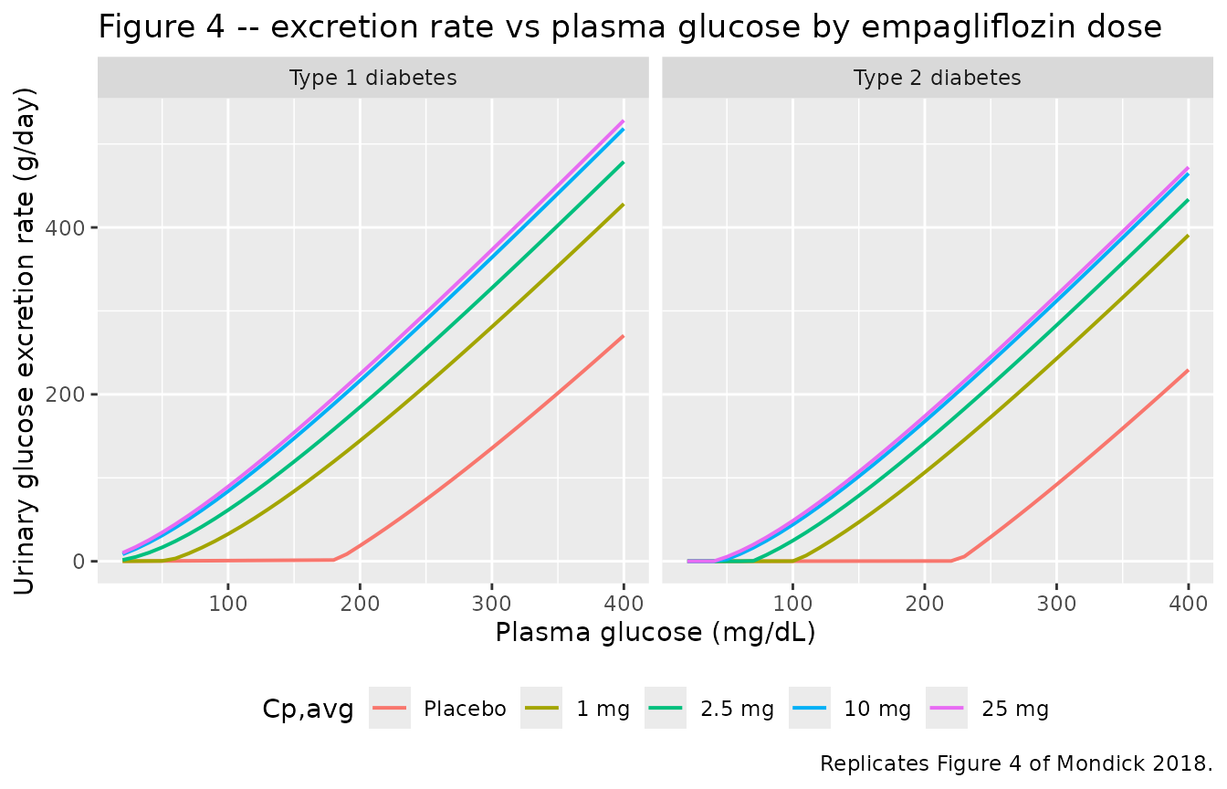
Three properties of this figure are asserted directly.
The sub-threshold leak. Below RTG the excretion rate
is exactly eGFR * iPG * (1 - FRAC) (equation 1). This is
the only check in the vignette that exercises FRAC, and it
is an exact identity, so it is asserted tightly.
EGFR_DL_H <- 102 * 1.95 / 1.73 * 0.6   # dL/h for the reference patient

leak <- fig4 |>
  dplyr::filter(treatment == "Placebo", pg_mgdl <= 150) |>
  dplyr::mutate(
    frac = ifelse(population == "Type 1 diabetes", 0.995, 0.999),
    predicted = EGFR_DL_H * pg_mgdl * (1 - frac) * 24 / 1000,
    rel_err = abs(uge_g_per_day - predicted) / predicted
  )

stopifnot(nrow(leak) > 0, max(leak$rel_err) < 1e-6)
The threshold. Because the sub-threshold leak is nonzero (and five times larger in T1DM, whose FRAC is 0.995 rather than 0.999), the plasma glucose at which a curve first exceeds a fixed excretion level is not itself the threshold. It should, however, sit just above the closed-form RTG. A 10 g/day level is used, which is well clear of the leak in both populations.
ONSET_G_DAY <- 10

onset <- fig4 |>
  dplyr::filter(uge_g_per_day > ONSET_G_DAY) |>
  dplyr::group_by(population, treatment) |>
  dplyr::summarise(onset_mgdl = min(pg_mgdl), .groups = "drop")

placebo_onset <- onset |> dplyr::filter(treatment == "Placebo")
rtg_placebo <- c("Type 1 diabetes" = 181, "Type 2 diabetes" = 225)
placebo_onset$rtg <- rtg_placebo[as.character(placebo_onset$population)]

stopifnot(
  nrow(placebo_onset) == 2L,
  # Above the threshold, and by no more than a modest margin.
  all(placebo_onset$onset_mgdl > placebo_onset$rtg),
  all(placebo_onset$onset_mgdl - placebo_onset$rtg <= 25)
)

# Mondick 2018 Results: "The lower RTG in patients with T1DM yields UGE at lower
# plasma glucose concentrations compared with patients with T2DM."
onset_wide <- onset |>
  tidyr::pivot_wider(names_from = population, values_from = onset_mgdl)
stopifnot(
  nrow(onset_wide) == nrow(rtg_key),
  all(onset_wide$`Type 1 diabetes` <= onset_wide$`Type 2 diabetes`)
)

# Excretion increases monotonically with dose wherever excretion is
# meaningful. The qualifier is necessary and is a property of the published
# model: equation 1 does not vanish as plasma glucose approaches the threshold
# from below, so in a narrow band just above its own (very low) threshold a
# high-dose arm can sit fractionally BELOW the sub-threshold leak of the arms
# still on equation 1. See "Errata and open questions".
mono <- fig4 |>
  dplyr::arrange(population, pg_mgdl, treatment) |>
  dplyr::group_by(population, pg_mgdl) |>
  dplyr::summarise(
    peak      = max(uge_g_per_day),
    worst_dip = min(diff(uge_g_per_day)),
    .groups   = "drop"
  )

stopifnot(
  nrow(mono) > 0,
  # Strictly monotone wherever any arm excretes more than 1 g/day.
  all(mono$worst_dip[mono$peak > 1] >= -1e-8),
  # And where it is not, the violation is a rounding-scale artefact of the
  # branch discontinuity, not a structural inversion.
  all(mono$worst_dip >= -0.5)
)

# How large the discontinuity artefact actually gets, in g/day.
round(min(mono$worst_dip), 4)
#> [1] -0.0111

onset_wide
#> # A tibble: 5 × 3
#>   treatment `Type 1 diabetes` `Type 2 diabetes`
#>   <fct>                 <dbl>             <dbl>
#> 1 Placebo                 200               240
#> 2 1 mg                     80               120
#> 3 2.5 mg                   40                90
#> 4 10 mg                    30                70
#> 5 25 mg                    20                60
Virtual cohort and PK simulation
The PK layer is validated on a virtual cohort matched to the EASE-1 demographics: 100 subjects per active dose arm, dosed once daily for 28 days, with dense sampling on day 1 and on day 28 plus a 72-hour washout (the paper collected ambulatory PK on days 29-31).
set.seed(20180501)

N_PER_ARM   <- 100
DOSES_MG    <- c("2.5 mg" = 2.5, "10 mg" = 10, "25 mg" = 25)
N_DOSES     <- 28
LAST_DOSE_H <- 24 * (N_DOSES - 1)   # 648 h

# Dense grid on day 1, on the day-28 interval, and through washout.
obs_times <- sort(unique(c(
  seq(0, 24, by = 0.25),
  seq(LAST_DOSE_H, LAST_DOSE_H + 24, by = 0.25),
  seq(LAST_DOSE_H + 24, LAST_DOSE_H + 96, by = 2)
)))

make_pk_cohort <- function(n, dose_mg, treatment, id_offset = 0L) {
  subj <- tibble(
    id  = id_offset + seq_len(n),
    # Mondick 2018 baseline demographics: BMI mean 25.6 (SD 3.69), age 41.0
    # (10.9), 71% male, eGFR 102 (13.8).
    BMI  = pmax(17, rnorm(n, 25.6, 3.69)),
    AGE  = pmin(60, pmax(20, rnorm(n, 41.0, 10.9))),
    SEXF = rbinom(n, 1, 0.293),
    CRCL = pmax(45, rnorm(n, 102, 13.8)),
    treatment = treatment
  ) |>
    # BSA is not reported by the paper; derive it from BMI with the Mosteller
    # formula at the cohort mean height (see "Assumptions and deviations").
    dplyr::mutate(
      HT_M = 1.75,
      BSA  = sqrt((BMI * HT_M^2) * (HT_M * 100) / 3600)
    ) |>
    dplyr::select(-HT_M)

  dosing <- subj |>
    tidyr::crossing(time = seq(0, LAST_DOSE_H, by = 24)) |>
    dplyr::mutate(
      amt = dose_mg, evid = 1L, cmt = "depot",
      # rate = -2 tells rxode2 to apply the model's dur(depot) zero-order window
      rate = -2, dvid = NA_integer_
    )

  obs <- subj |>
    tidyr::crossing(time = obs_times) |>
    # dvid = 1 selects the Cc endpoint of this multi-endpoint model.
    dplyr::mutate(amt = NA_real_, evid = 0L, cmt = "central", rate = 0, dvid = 1L)

  dplyr::bind_rows(dosing, obs) |>
    dplyr::mutate(GLU = 8) |>   # PK layer is independent of plasma glucose
    dplyr::arrange(id, time, dplyr::desc(evid))
}

pk_events <- dplyr::bind_rows(
  make_pk_cohort(N_PER_ARM, DOSES_MG[["2.5 mg"]], "2.5 mg", id_offset =   0L),
  make_pk_cohort(N_PER_ARM, DOSES_MG[["10 mg"]],  "10 mg",  id_offset = 100L),
  make_pk_cohort(N_PER_ARM, DOSES_MG[["25 mg"]],  "25 mg",  id_offset = 200L)
)

stopifnot(!anyDuplicated(unique(pk_events[, c("id", "time", "evid")])))
pk_sim <- rxode2::rxSolve(
  mod_t1dm,
  events = pk_events,
  keep = c("treatment"),
  useLinCmt = FALSE
) |>
  as.data.frame()
#> ℹ parameter labels from comments will be replaced by 'label()'

if (is.null(pk_sim$id)) pk_sim$id <- 1L
Figure 2 – day 1 concentration-time profile
pk_sim |>
  dplyr::filter(time <= 24, time > 0) |>
  dplyr::group_by(treatment, time) |>
  dplyr::summarise(
    Q05 = quantile(Cc, 0.05), Q50 = median(Cc), Q95 = quantile(Cc, 0.95),
    .groups = "drop"
  ) |>
  dplyr::mutate(treatment = factor(treatment, levels = names(DOSES_MG))) |>
  ggplot(aes(time, Q50)) +
  geom_ribbon(aes(ymin = Q05, ymax = Q95), alpha = 0.25) +
  geom_line() +
  facet_wrap(~treatment) +
  scale_y_log10() +
  labs(
    x = "Time (h)", y = "Empagliflozin (nmol/L)",
    title = "Figure 2 -- day 1 empagliflozin concentrations",
    caption = "Replicates Figure 2 of Mondick 2018 (median with 5th-95th percentiles)."
  )
#> Warning in scale_y_log10(): log-10 transformation introduced infinite values.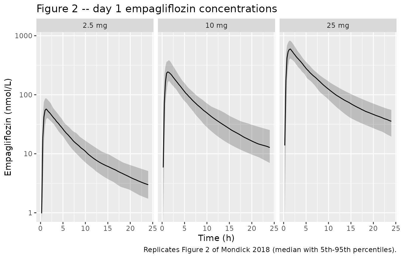
PKNCA validation
sim_nca <- pk_sim |>
  dplyr::filter(!is.na(Cc)) |>
  dplyr::select(id, time, Cc, treatment)

# Guarantee a time-zero record per subject; pre-dose Cc is 0 for an oral dose.
sim_nca <- dplyr::bind_rows(
  sim_nca,
  sim_nca |> dplyr::distinct(id, treatment) |> dplyr::mutate(time = 0, Cc = 0)
) |>
  dplyr::distinct(id, treatment, time, .keep_all = TRUE) |>
  dplyr::arrange(id, treatment, time)

conc_obj <- PKNCA::PKNCAconc(sim_nca, Cc ~ time | treatment + id)

dose_df <- pk_events |>
  dplyr::filter(evid == 1L) |>
  dplyr::select(id, time, amt, treatment)

dose_obj <- PKNCA::PKNCAdose(dose_df, amt ~ time | treatment + id)

intervals <- data.frame(
  start     = c(LAST_DOSE_H, LAST_DOSE_H),
  end       = c(LAST_DOSE_H + 24, Inf),
  cmax      = c(TRUE,  FALSE),
  tmax      = c(TRUE,  FALSE),
  auclast   = c(TRUE,  FALSE),
  cav       = c(TRUE,  FALSE),
  half.life = c(FALSE, TRUE)
)

nca_res <- PKNCA::pk.nca(PKNCA::PKNCAdata(conc_obj, dose_obj, intervals = intervals))

# PKNCA emits some bookkeeping parameters (tlast, lambda.z, ...) for BOTH
# intervals, so the interval must stay in the key or pivot_wider silently
# produces list-columns. Take the within-interval parameters from the dosing
# interval and half-life from the terminal one.
nca_long <- as.data.frame(nca_res) |>
  dplyr::select(treatment, id, start, end, PPTESTCD, PPORRES)

nca_wide <- nca_long |>
  dplyr::filter(end == LAST_DOSE_H + 24,
                PPTESTCD %in% c("cmax", "tmax", "auclast", "cav")) |>
  dplyr::select(treatment, id, PPTESTCD, PPORRES) |>
  tidyr::pivot_wider(names_from = PPTESTCD, values_from = PPORRES) |>
  dplyr::left_join(
    nca_long |>
      dplyr::filter(is.infinite(end), PPTESTCD == "half.life") |>
      dplyr::select(treatment, id, half.life = PPORRES),
    by = c("treatment", "id")
  )

stopifnot(nrow(nca_wide) == 3L * N_PER_ARM,
          !anyNA(nca_wide$cav), !anyNA(nca_wide$auclast))
The simulated steady-state exposures, before comparison with the paper:
# PKNCA reports tmax relative to the dose that opens the interval, so it is
# already a time since the day-28 dose and must NOT have LAST_DOSE_H subtracted.
stopifnot(all(nca_wide$tmax >= 0), all(nca_wide$tmax <= 24))

nca_wide |>
  dplyr::mutate(treatment = factor(treatment, levels = names(DOSES_MG))) |>
  dplyr::group_by(treatment) |>
  dplyr::summarise(
    cmax = median(cmax), tmax = median(tmax),
    auclast = median(auclast), cav = median(cav),
    half.life = median(half.life, na.rm = TRUE), .groups = "drop"
  ) |>
  dplyr::mutate(dplyr::across(where(is.numeric), \(x) signif(x, 3))) |>
  dplyr::rename(
    "Dose"                       = treatment,
    "Cmax (nmol/L)"              = cmax,
    "Tmax (h post-dose)"         = tmax,
    "AUCtau (nmol*h/L)"          = auclast,
    "Cavg (nmol/L)"              = cav,
    "Terminal t1/2 (h)"          = half.life
  ) |>
knitr::kable(caption = "Median simulated steady-state NCA on the day-28 dosing interval.")| Dose | Cmax (nmol/L) | Tmax (h post-dose) | AUCtau (nmol*h/L) | Cavg (nmol/L) | Terminal t1/2 (h) |
|---|---|---|---|---|---|
| 2.5 mg | 62.5 | 1.25 | 407 | 17 | 12.9 |
| 10 mg | 270.0 | 1.25 | 1700 | 71 | 12.7 |
| 25 mg | 660.0 | 1.25 | 4470 | 186 | 12.6 |
Per-subject structural identity: AUCtau = Dose / CL
For linear PK at steady state the area under one dosing interval is
exactly Dose / CL. Because both sides use the same drawn
parameters, this is a pure numerical-accuracy check and can be asserted
tightly per subject.
subj_cl <- pk_sim |>
  dplyr::group_by(id, treatment) |>
  dplyr::summarise(cl = dplyr::first(cl), .groups = "drop")

ident <- nca_wide |>
  dplyr::left_join(subj_cl, by = c("id", "treatment")) |>
  dplyr::mutate(
    dose_nmol = DOSES_MG[as.character(treatment)] / MW_EMPA * 1e6,
    auc_pred  = dose_nmol / cl,
    pct_diff  = 100 * (auclast - auc_pred) / auc_pred
  )

stopifnot(
  nrow(ident) == 3L * N_PER_ARM,
  !anyNA(ident$pct_diff),
  # auclast under-reads AUCtau only by trapezoidal error on a fine grid.
  max(abs(ident$pct_diff)) < 1.0
)

summary(ident$pct_diff)
#>       Min.    1st Qu.     Median       Mean    3rd Qu.       Max.
#> -0.1387484 -0.0273978 -0.0126081 -0.0136998 -0.0001973  0.0886920
Comparison against the published steady-state exposures
Mondick 2018 reports the average steady-state plasma concentration it
paired with each RTG value. cav from PKNCA is the same
quantity (AUCtau / tau).
published <- tibble::tribble(
  ~treatment, ~cav,
  "2.5 mg",   21.5,
  "10 mg",    85.8,
  "25 mg",   215.0
)

cmp <- nlmixr2lib::ncaComparisonTable(
  simulated     = nca_res,
  reference     = published,
  by            = "treatment",
  # Restrict to the one quantity the paper reports; without this the two NCA
  # intervals both contribute bookkeeping parameters.
  params        = "cav",
  units         = c(cav = "nmol/L"),
  tolerance_pct = 20
)

knitr::kable(
  cmp,
  caption = paste(
    "Simulated steady-state NCA vs the average concentrations reported in",
    "Mondick 2018. * differs from the reference by more than 20%."
  )
)| NCA parameter | treatment | Reference | Simulated | % diff |
|---|---|---|---|---|
| Cavg (nmol/L) | 2.5 mg | 21.5 | 17 | -21.1%* |
| Cavg (nmol/L) | 10 mg | 85.8 | 71 | -17.2% |
| Cavg (nmol/L) | 25 mg | 215 | 186 | -13.5% |
Every published average sits above the simulation. The well-defined
way to size that gap is against the typical value
Dose / (CL/F * tau), which is free of sampling noise: the
ratio is 1.145, 1.142 and 1.145 at 2.5, 10 and 25 mg. A single common
factor across a three-fold and then ten-fold dose increment is a scale
difference, not a transcription error in any one row – the published
averages correspond to an apparent clearance near 10.7 L/h rather than
the 12.3 L/h of Supplementary Table 1. See “Errata and open questions”;
no parameter has been adjusted.
The simulated medians carry an additional, uninteresting spread: each dose arm draws its own 100 subjects, so each has its own median CL/F (roughly 12.4 to 13.6 L/h here). The check below therefore separates the two effects – the published-vs-typical ratio is asserted tightly, while the simulated medians are asserted against the exact linear-PK identity for their own arm’s median clearance.
TAU_H <- 24

offset <- published |>
  dplyr::mutate(
    dose_nmol = DOSES_MG[as.character(treatment)] / MW_EMPA * 1e6,
    # Deterministic typical-value average concentration, Dose / (CL/F * tau).
    cav_typical = dose_nmol / (exp(ui_t1dm$theta[["lcl"]]) * TAU_H),
    ratio_typical = cav / cav_typical
  ) |>
  dplyr::left_join(
    nca_wide |>
      dplyr::left_join(subj_cl, by = c("id", "treatment")) |>
      dplyr::group_by(treatment) |>
      dplyr::summarise(cav_sim = median(cav), cl_arm = median(cl), .groups = "drop"),
    by = "treatment"
  ) |>
  dplyr::mutate(
    ratio_sim   = cav / cav_sim,
    # Exact linear-PK expectation for THIS arm's sampled subjects.
    cav_from_cl = dose_nmol / (cl_arm * TAU_H)
  )

stopifnot(
  nrow(offset) == 3L, !anyNA(offset$ratio_sim),
  # Against the typical value this is exact arithmetic, so the claim that the
  # offset is ONE scale factor rather than a per-dose discrepancy is asserted
  # tightly.
  diff(range(offset$ratio_typical)) < 0.01,
  # The published averages imply an apparent clearance near 10.7 L/h.
  abs(exp(ui_t1dm$theta[["lcl"]]) / mean(offset$ratio_typical) - 10.7) < 0.2,
  # Each arm's median Cavg IS Dose / (arm median CL * tau). This is an exact
  # identity, so the residual spread in ratio_sim is entirely per-arm sampling
  # of CL/F and carries no information about the published offset.
  max(abs(offset$cav_sim / offset$cav_from_cl - 1)) < 0.01
)

offset |>
  dplyr::mutate(dplyr::across(where(is.numeric), \(x) signif(x, 4))) |>
  dplyr::select(treatment, cav, cav_typical, ratio_typical,
                cl_arm, cav_sim, cav_from_cl, ratio_sim) |>
  dplyr::rename(
    "Dose"                          = treatment,
    "Published Cavg (nmol/L)"       = cav,
    "Dose/(CL*tau) (nmol/L)"        = cav_typical,
    "Published / typical"           = ratio_typical,
    "Arm median CL/F (L/h)"         = cl_arm,
    "Simulated median Cavg"         = cav_sim,
    "Dose/(arm CL*tau)"             = cav_from_cl,
    "Published / simulated"         = ratio_sim
  ) |>
knitr::kable(caption = "Decomposition of the published-vs-simulated Cavg offset.")| Dose | Published Cavg (nmol/L) | Dose/(CL*tau) (nmol/L) | Published / typical | Arm median CL/F (L/h) | Simulated median Cavg | Dose/(arm CL*tau) | Published / simulated |
|---|---|---|---|---|---|---|---|
| 2.5 mg | 21.5 | 18.78 | 1.145 | 13.62 | 16.96 | 16.97 | 1.267 |
| 10 mg | 85.8 | 75.13 | 1.142 | 13.01 | 71.01 | 71.01 | 1.208 |
| 25 mg | 215.0 | 187.80 | 1.145 | 12.42 | 186.00 | 186.00 | 1.156 |
Validation 3 – covariate and population effects on 24-hour UGE
Figure 3 of Mondick 2018 compares typical 24-hour steady-state UGE between the reference patient and (a) female patients, (b) the extremes of the study age range, in each population. The paper’s own design for the T1DM-vs-T2DM comparison fed both populations the same median plasma-glucose profile, so the ordering claims can be reproduced exactly even though the profile itself is not published.
A single diurnal profile is used for every arm here; see “Assumptions and deviations” for its construction.
# Eight-point diurnal profile, mmol/L. Mondick 2018 collected 8-point plasma
# glucose profiles but does not publish the medians, so this is an assumed
# clinically plausible T1DM shape, NOT a transcription from the paper.
pg_profile <- tibble::tribble(
  ~time, ~GLU,
    0.0,  8.0,   # pre-breakfast
    1.5, 12.5,   # post-breakfast peak
    4.0,  8.5,   # pre-lunch
    5.5, 12.0,   # post-lunch peak
    8.0,  8.0,   # pre-dinner
    9.5, 11.5,   # post-dinner peak
   12.0,  9.0,   # bedtime
   24.0,  8.0    # next pre-breakfast
)

# Mean over the day by the same linear interpolation the model uses.
pg_mean_mgdl <- with(
  pg_profile,
  sum(diff(time) * (head(GLU, -1) + tail(GLU, -1)) / 2) / 24
) * 18.016
round(pg_mean_mgdl, 1)
#> [1] 168.3
# Typical-value arms: one subject per (dose x sex x age) cell, random effects
# zeroed, so each row is exactly the typical prediction the paper plots.
uge_arms <- tidyr::crossing(
  rtg_key |> dplyr::select(treatment, dose_mg = cavg_nM),
  SEXF = c(0, 1),
  AGE  = c(20, 42, 58, 60)
) |>
  dplyr::mutate(
    dose_mg = dplyr::recode(
      treatment,
      "Placebo" = 0, "1 mg" = 1, "2.5 mg" = 2.5, "10 mg" = 10, "25 mg" = 25
    ),
    id = dplyr::row_number(),
    BMI = 25.6, CRCL = 102, BSA = 1.95
  )

UGE_DAYS <- 10   # QD dosing reaches steady state within ~3 days

uge_dosing <- uge_arms |>
  tidyr::crossing(time = seq(0, 24 * (UGE_DAYS - 1), by = 24)) |>
  dplyr::mutate(amt = dose_mg, evid = 1L, cmt = "depot", rate = -2,
                dvid = NA_integer_) |>
  dplyr::filter(amt > 0)

# Observation rows carry the repeating daily glucose profile, plus the day
# boundaries needed to difference the cumulative excretion state.
uge_obs <- uge_arms |>
  tidyr::crossing(day = seq_len(UGE_DAYS) - 1L, pg_profile) |>
  dplyr::mutate(time = day * 24 + time) |>
  dplyr::select(-day) |>
  dplyr::bind_rows(
    uge_arms |> tidyr::crossing(time = c(24 * (UGE_DAYS - 1), 24 * UGE_DAYS)) |>
      dplyr::mutate(GLU = 8.0)
  ) |>
  dplyr::mutate(amt = NA_real_, evid = 0L, cmt = "central", rate = 0,
                dvid = 1L) |>
  dplyr::distinct(id, time, .keep_all = TRUE)

uge_events <- dplyr::bind_rows(uge_dosing, uge_obs) |>
  dplyr::arrange(id, time, dplyr::desc(evid)) |>
  tidyr::fill(GLU, .direction = "downup")

stopifnot(!anyDuplicated(unique(uge_events[, c("id", "time", "evid")])))
solve_uge <- function(mod, label) {
  rxode2::rxSolve(
    mod |> rxode2::zeroRe(),
    events = uge_events,
    keep = c("treatment", "SEXF", "AGE"),
    omega = NA,
    useLinCmt = FALSE
  ) |>
    as.data.frame() |>
    dplyr::filter(time %in% c(24 * (UGE_DAYS - 1), 24 * UGE_DAYS)) |>
    dplyr::group_by(id, treatment, SEXF, AGE) |>
    # 24-hour UGE = the increment of the cumulative state over the last day.
    dplyr::summarise(uge_g = (max(UGE) - min(UGE)) / 1000, .groups = "drop") |>
    dplyr::mutate(population = label)
}

uge <- dplyr::bind_rows(
  solve_uge(mod_t1dm, "Type 1 diabetes"),
  solve_uge(mod_t2dm, "Type 2 diabetes")
)
#> ℹ parameter labels from comments will be replaced by 'label()'
#> Warning: multi-subject simulation without without 'omega'
#> ℹ parameter labels from comments will be replaced by 'label()'
#> Warning: multi-subject simulation without without 'omega'

# Placebo-corrected increase, matching the paper's reported quantity.
uge_pc <- uge |>
  dplyr::group_by(population, SEXF, AGE) |>
  dplyr::mutate(uge_pc_g = uge_g - uge_g[treatment == "Placebo"]) |>
  dplyr::ungroup() |>
  dplyr::filter(treatment != "Placebo")
uge_pc |>
  dplyr::filter(treatment == "25 mg", AGE %in% c(42, 58)) |>
  dplyr::filter((population == "Type 1 diabetes" & AGE == 42) |
                (population == "Type 2 diabetes" & AGE == 58)) |>
  dplyr::transmute(
    population,
    sex = ifelse(SEXF == 1, "Female", "Male"),
    age = AGE,
    uge_pc_g = round(uge_pc_g, 1)
  ) |>
  dplyr::rename(
    "Population"                             = population,
    "Sex"                                    = sex,
    "Age (years)"                            = age,
    "Placebo-corrected 24-h UGE, 25 mg (g)"  = uge_pc_g
  ) |>
  knitr::kable(
    caption = paste(
      "Typical placebo-corrected 24-hour urinary glucose excretion at",
      "empagliflozin 25 mg, at each population's reference patient.",
      "Mondick 2018 reports 105.6 g (male) and 88.9 g (female) for T1DM and",
      "84.7 g (male) and 66.9 g (female) for T2DM, computed with the",
      "unpublished median plasma-glucose profiles."
    )
)| Population | Sex | Age (years) | Placebo-corrected 24-h UGE, 25 mg (g) |
|---|---|---|---|
| Type 1 diabetes | Male | 42 | 169.7 |
| Type 1 diabetes | Female | 42 | 139.7 |
| Type 2 diabetes | Male | 58 | 127.7 |
| Type 2 diabetes | Female | 58 | 106.3 |
The absolute magnitudes are not directly comparable with the paper’s, because they scale with the plasma-glucose profile that drives filtration and that profile is not published. The ordering claims are, and they are asserted here.
ref <- uge_pc |>
  dplyr::filter(treatment == "25 mg") |>
  dplyr::filter((population == "Type 1 diabetes" & AGE == 42) |
                (population == "Type 2 diabetes" & AGE == 58))

get_uge <- function(pop, sexf) {
  v <- ref$uge_pc_g[ref$population == pop & ref$SEXF == sexf]
  if (length(v) != 1L) stop("no unique row for ", pop, " SEXF=", sexf)
  v
}

t1_m <- get_uge("Type 1 diabetes", 0); t1_f <- get_uge("Type 1 diabetes", 1)
t2_m <- get_uge("Type 2 diabetes", 0); t2_f <- get_uge("Type 2 diabetes", 1)

stopifnot(
  # "female patients had a reduced cumulative UGE compared with the reference
  #  patient" -- in both populations.
  t1_f < t1_m,
  t2_f < t2_m,
  # "patients with T1DM exhibit increased 24-hour UGE compared with T2DM"
  t1_m > t2_m,
  t1_f > t2_f,
  # "UGE in female patients with T1DM was still greater than that in male
  #  patients with T2DM."
  t1_f > t2_m,
  # Every excretion is positive and finite.
  all(is.finite(uge_pc$uge_pc_g)), all(uge_pc$uge_pc_g > 0)
)

# The paper's female:male ratios are 88.9/105.6 = 0.842 (T1DM) and
# 66.9/84.7 = 0.790 (T2DM). These are ratios of the same simulation and so are
# far less sensitive to the glucose profile than the absolute values.
ratios <- c(t1dm = t1_f / t1_m, t2dm = t2_f / t2_m)
round(ratios, 3)
#>  t1dm  t2dm
#> 0.824 0.832
stopifnot(abs(ratios[["t1dm"]] - 0.842) < 0.10,
          abs(ratios[["t2dm"]] - 0.790) < 0.10)

# "UGE in patients with T1DM was similar across extremes of age with all doses
# of empagliflozin." Asserted as a modest spread across the 20-60 year study
# range; the exact spread depends on the assumed glucose profile.
age_span <- uge_pc |>
  dplyr::filter(treatment == "25 mg", SEXF == 0, AGE %in% c(20, 60)) |>
  dplyr::group_by(population) |>
  dplyr::summarise(span = max(uge_pc_g) / min(uge_pc_g), .groups = "drop")
stopifnot(nrow(age_span) == 2L, all(age_span$span < 1.30))
age_span
#> # A tibble: 2 × 2
#>   population       span
#>   <chr>           <dbl>
#> 1 Type 1 diabetes  1.06
#> 2 Type 2 diabetes  1.24
Supplementary Figure 4 makes the sharper, glucose-independent version
of the same claim: every covariate effect on Gmax and
Imax lies inside a “minimal effect region” of 80% to 125%
of the reference-patient value. That is a property of the parameters
alone, so it can be checked exactly.
rel_effects <- function(ui, ref_age) {
  th <- function(nm) ui$theta[[nm]]
  ages <- c(20, 60)
  tibble::tibble(
    effect = c("Gmax, age 20", "Gmax, age 60", "Gmax, female",
               "Imax, age 20", "Imax, age 60", "Imax, female"),
    relative = c(
      (ages / ref_age)^th("e_age_gmax"), th("e_sexf_gmax"),
      (ages / ref_age)^th("e_age_imax"), th("e_sexf_imax")
    )
  )
}

minimal_effect <- dplyr::bind_rows(
  rel_effects(ui_t1dm, 42) |> dplyr::mutate(population = "Type 1 diabetes"),
  rel_effects(ui_t2dm, 58) |> dplyr::mutate(population = "Type 2 diabetes")
)

stopifnot(
  nrow(minimal_effect) == 12L,
  all(minimal_effect$relative >= 0.80),
  all(minimal_effect$relative <= 1.25)
)

minimal_effect |>
  tidyr::pivot_wider(names_from = population, values_from = relative) |>
  dplyr::mutate(dplyr::across(where(is.numeric), \(x) round(x, 3))) |>
  knitr::kable(
    caption = paste(
      "Relative covariate effects vs each population's reference patient.",
      "Mondick 2018 Supplementary Figure 4 reports all of these inside a",
      "minimal-effect region of 80% to 125%."
    )
)| effect | Type 1 diabetes | Type 2 diabetes |
|---|---|---|
| Gmax, age 20 | 1.015 | 1.061 |
| Gmax, age 60 | 0.993 | 0.998 |
| Gmax, female | 1.130 | 1.120 |
| Imax, age 20 | 0.967 | 1.198 |
| Imax, age 60 | 1.016 | 0.994 |
| Imax, female | 0.901 | 0.984 |
Inverting the answer key: what plasma glucose reproduces 105.6 g?
The model, the paper’s 105.6 g and the cohort-mean renal function together pin the mean plasma glucose that the paper’s own T1DM 25 mg simulation must have used. Recovering it is a dimensional check on the whole filtration arm: an implausible answer would mean a unit error somewhere.
uge_at_constant_pg <- function(mod, pg_mgdl_vec, dose_mg = 25, age = 42, sexf = 0) {
  subj <- tibble(
    id = seq_along(pg_mgdl_vec),
    pg_mgdl = pg_mgdl_vec,
    AGE = age, SEXF = sexf, BMI = 25.6, CRCL = 102, BSA = 1.95
  ) |>
    dplyr::mutate(GLU = pg_mgdl / 18.016)

  dosing <- subj |>
    tidyr::crossing(time = seq(0, 24 * (UGE_DAYS - 1), by = 24)) |>
    dplyr::mutate(amt = dose_mg, evid = 1L, cmt = "depot", rate = -2,
                  dvid = NA_integer_) |>
    dplyr::filter(amt > 0)

  # Only the two day boundaries are needed to difference the cumulative state;
  # plasma glucose is constant per subject so no intermediate rows are required.
  obs <- subj |>
    tidyr::crossing(time = c(24 * (UGE_DAYS - 1), 24 * UGE_DAYS)) |>
    dplyr::mutate(amt = NA_real_, evid = 0L, cmt = "central", rate = 0,
                  dvid = 1L)

  ev <- dplyr::bind_rows(dosing, obs) |>
    dplyr::arrange(id, time, dplyr::desc(evid))

  rxode2::rxSolve(mod |> rxode2::zeroRe(), events = ev, keep = c("pg_mgdl"),
                  omega = NA, useLinCmt = FALSE) |>
    as.data.frame() |>
    dplyr::filter(time %in% c(24 * (UGE_DAYS - 1), 24 * UGE_DAYS)) |>
    dplyr::group_by(id, pg_mgdl) |>
    dplyr::summarise(uge_g = (max(UGE) - min(UGE)) / 1000, .groups = "drop")
}

pg_scan <- seq(60, 260, by = 5)
drug_curve    <- uge_at_constant_pg(mod_t1dm, pg_scan, dose_mg = 25)
#> ℹ parameter labels from comments will be replaced by 'label()'
#> Warning: multi-subject simulation without without 'omega'
placebo_curve <- uge_at_constant_pg(mod_t1dm, pg_scan, dose_mg = 0)
#> ℹ parameter labels from comments will be replaced by 'label()'
#> Warning: multi-subject simulation without without 'omega'

pc_curve <- drug_curve |>
  dplyr::rename(uge_drug = uge_g) |>
  dplyr::left_join(placebo_curve |> dplyr::select(pg_mgdl, uge_pbo = uge_g),
                   by = "pg_mgdl") |>
  dplyr::mutate(uge_pc = uge_drug - uge_pbo)

# Placebo-corrected UGE is monotone in plasma glucose, so the inverse is unique.
stopifnot(all(diff(pc_curve$uge_pc) > 0))
pg_implied <- approx(pc_curve$uge_pc, pc_curve$pg_mgdl, xout = 105.6)$y
round(pg_implied, 1)
#> [1] 117

# A mean plasma glucose in the range achievable on insulin plus an SGLT2
# inhibitor. Well outside 60-260 mg/dL would indicate a unit error.
stopifnot(is.finite(pg_implied), pg_implied > 80, pg_implied < 200)
The implied mean plasma glucose is a clinically attainable
on-treatment value for insulin-treated T1DM, so the filtration arm
carries no unit error. As an independent dimensional check, the model’s
maximum renal reabsorption capacity eGFR * Gmax for this
patient is:
Assumptions and deviations
-
Plasma-glucose profiles are not published. Mondick
2018 fitted 8-point daily plasma-glucose profiles and used the median
profile per dose group as model input, but reports neither the medians
nor the sampling times. The diurnal profile in the
glucose-profilechunk is an assumed, clinically plausible T1DM shape. Every absolute UGE number in this vignette therefore depends on that assumption; the validations that matter are stated as exact reproductions of published quantities (RTG, Figure 4) or as ordering / ratio claims that are insensitive to the profile. - A single common glucose profile is used for both populations. This matches the paper’s own design: “The median plasma glucose profile from each empagliflozin dose group in the study in patients with T1DM was used as input, irrespective of the patient population, to ensure that differences did not result from differences in plasma glucose sampling.”
- Body surface area. The model needs BSA to convert the BSA-normalized eGFR back to an absolute filtration rate, but Mondick 2018 reports no BSA distribution. The virtual cohort derives BSA from each subject’s BMI with the Mosteller formula at a fixed 1.75 m height; the typical-value arms use BSA = 1.95 m^2, the Du Bois value for the cohort’s mean weight (79.3 kg) at that height.
-
Non-paper-derived value: empagliflozin molar mass.
MW_EMPA = 450.91 g/mol(formula C23H27ClO7) is not reported in the paper. It appears in both model files asmwEmpaand is used only to let doses be given in mg while concentrations and IC50 are expressed in the paper’s nmol/L. Apparent clearance and volume are unit-invariant, so this is exactly equivalent to dosing in nmol; no fitted quantity depends on it. -
Glucose unit conversion. The
GLUcovariate register is canonically in mmol/L while the paper works throughout in mg/dL. Both model files convert internally with 18.016 mg/dL per mmol/L (glucose molar mass 180.16 g/mol), the same factor already used byBosch_2025_glp1ra_hba1c.R. - Cohort demographics are drawn independently from the reported marginal means and SDs (BMI, age, eGFR) with truncation at the study limits. The paper states only that “age and eGFR distributions were relatively comparable between male and female patients, and men were slightly heavier than women (data not shown)”, so no correlation structure is imposed.
-
Typical-value arms. The Figure 3 comparison in the
paper is a Monte Carlo median over a cohort carrying IIV and residual
variability. Here the corresponding quantity is computed with
rxode2::zeroRe()at one subject per covariate cell, which is the typical-value prediction. For the ratio and ordering claims asserted above the two agree; absolute medians under large IIV on a nonlinear response would not necessarily. -
useLinCmt = FALSEis passed to everyrxSolve()call. Both models are multi-output (CcandUGE) over four ODE states, and rxode2’s automatic ODE-to-linCmt()conversion corrupts the endpoint mapping for that shape.
Errata and open questions
-
Theta indices for the BMI exponents disagree between the
main text and the supplement. The main-text PK equations
(p.644) attach
theta_10to Vp/F andtheta_11to Q/F; Supplementary Table 1 attachestheta_10to Q/F (1.77) andtheta_11to Vp/F (0.775). Only the index labels conflict. The table states the parameter name and its value on the same row, so the value-to-parameter binding is unambiguous from the table alone, and that binding is what both model files encode:(BMI/25)^1.77on Q/F and(BMI/25)^0.775on Vp/F. -
The Supplementary Table 2 “Model” column prints
1 + thetawhere the main-text equations print1 - theta. The logistic transforms for FRAC and Imax are rendered in the supplement asexp(LN(theta/(1+theta)+eta)) / (1+exp(LN(theta/(1+theta)+eta))). The main-text equations on p.643 giveln(theta/(1-theta)) + eta, which is the ordinary logit and is the only form that returns the tabulated estimates (expit(logit(0.995)) = 0.995); the supplement’s version would returntheta/(1+2*theta) = 0.332. The1 - thetaform is used. This is consistent with a minus sign lost in the supplement’s equation rendering. -
Published steady-state Cp,avg values are ~14.5% higher than
Dose / (CL/F * tau). The offset is essentially identical at 1, 2.5, 10 and 25 mg (1.145, 1.145, 1.142, 1.145), so it is a single scale factor and not a transcription error in an individual row; it corresponds to an apparent clearance near 10.7 L/h rather than the 12.3 L/h of Supplementary Table 1. Mondick 2018 does not say how the average concentrations were derived, and 10.7 L/h is close to the empagliflozin CL/F reported for the larger T2DM populations the paper cites (references 21 and 25). Because the RTG values are quoted against those concentrations, the RTG answer key in Validation 1 is reproduced by driving the model to the published concentrations rather than by dosing; no parameter has been altered. -
The T2DM parameter set is transcribed from a secondary
source. Mondick 2018 Supplementary Table 2 reproduces the
complete Mondick 2016 (Diabetes Obes Metab 18:241-248) parameter set,
including covariate effects, the IIV block and residual error, and the
2018 paper uses it for its own Figures 4 and 5. That primary paper was
not available when this model was built, so
Mondick_2018_empagliflozin_t2dmshould be re-verified against it if it is acquired. The T2DM file also has no PK layer of its own: it reuses the T1DM PK parameters, which is the pairing the authors themselves used (“the PK parameter estimates from the analysis presented here were used to simulate PK profiles for both populations”). -
The T2DM cohort size and demographics are not
restated in Mondick 2018, so
population$n_subjectsisNAin the T2DM model file. -
Age effects are retained at their published point
estimates even though both 95% CIs span zero and the paper
concludes that “no influence of age on Gmax and Imax could be
identified”. They are part of the reported full covariate model, so they
are encoded rather than dropped; a user who wants the paper’s conclusion
can set
e_age_gmaxande_age_imaxto zero. -
The excretion rate is discontinuous at the branch
point between equations 1 and 2, by
eGFR * RTG * (1 - FRAC). This is a property of the published model, not of the encoding: the sub-threshold leak term does not vanish as plasma glucose approaches the threshold from below. At the T1DM reference patient the jump is about 1.5 g/day against an on-treatment excretion of order 100 g/day. It has one visible consequence in the Figure 4 replication: in a narrow band of plasma glucose just above a high-dose arm’s (very low) threshold, that arm has crossed onto equation 2 and is excreting from essentially zero, while the lower-dose arms are still on equation 1 and excreting their constant leak. Excretion is therefore not strictly monotone in dose across that band – at the T2DM reference patient and 40 mg/dL plasma glucose the 25 mg arm sits 0.011 g/day below the placebo arm. The magnitude is negligible (three to four orders of magnitude below on-treatment excretion), and thefigure-4-assertchunk asserts monotonicity wherever any arm excretes more than 1 g/day while separately bounding the artefact.