Doravirine (Vaddady 2020)
Source:vignettes/articles/Vaddady_2020_doravirine.Rmd
Vaddady_2020_doravirine.RmdModel and source
- Citation: Vaddady P, Kandala B, Yee KL. Population Pharmacokinetic and Pharmacodynamic Analysis To Evaluate a Switch to Doravirine/Lamivudine/Tenofovir Disoproxil Fumarate in People Living with HIV-1. Antimicrob Agents Chemother. 2020;64(11):e00590-20. doi:10.1128/AAC.00590-20. Covariate-equation forms and the residual-error structure are those of the predecessor model it re-estimates: Yee KL, Ouerdani A, Claussen A, de Greef R, Wenning L. Population Pharmacokinetics of Doravirine and Exposure-Response Analysis in Individuals with HIV-1. Antimicrob Agents Chemother. 2019;63(4):e02502-18. doi:10.1128/AAC.02502-18.
- Description: One-compartment population PK model with first-order absorption for oral doravirine in healthy participants, treatment-naive adults with HIV-1, and virologically suppressed adults with HIV-1 switching to doravirine/lamivudine/tenofovir disoproxil fumarate (DRIVE-SHIFT immediate-switch group); linear age effect on CL/F, linear weight and healthy-versus-HIV-1 effects on V/F, and dose-band relative bioavailability
- Article: https://doi.org/10.1128/AAC.00590-20 (open access; parameter estimates are in Supplemental Table S1 of the online supplement)
- Predecessor model (source of the covariate-equation forms and the residual-error structure): https://doi.org/10.1128/AAC.02502-18
Vaddady 2020 re-estimated the doravirine population PK model of Yee 2019 after adding the sparse PK data of the DRIVE-SHIFT immediate-switch group (ISG; people living with HIV-1 who were virologically suppressed on another regimen and switched to doravirine/lamivudine/tenofovir disoproxil fumarate). The structure and covariates are unchanged from Yee 2019; only the estimates move slightly. This file packages the Vaddady 2020 re-estimate.
The paper’s exposure-response analysis (logistic regression of week-48 virologic response on steady-state C24) found slopes not different from zero and reports no slope estimates, so there is no PD component to package.
Population
The analysis data set pooled 341 healthy participants from phase 1 trials, 959 treatment-naive participants with HIV-1 (phase 1b, the phase 2b trial P007 and the phase 3 trials P018 DRIVE-FORWARD and P021 DRIVE-AHEAD), and 443 virologically suppressed participants with HIV-1 from the DRIVE-SHIFT (P024) ISG, for 1,743 participants in total (1,402 with HIV-1). Doses ranged from 6 to 200 mg in phase 1, 25 to 200 mg once daily in phase 2b, and 100 mg once daily in phase 3. Vaddady 2020 does not tabulate the demographics of the combined set; Yee 2019 Table 1 reports 80.8% male and 65.2% White, 21.6% Black and 6.7% Asian for the original 1,300 participants, and the covariate equations are centred on the median age (34 years) and a reference weight of 75 kg.
str(readModelDb("Vaddady_2020_doravirine")()$population)
#> List of 11
#>  $ species       : chr "human"
#>  $ n_subjects    : int 1743
#>  $ n_studies     : int 24
#>  $ age_median    : chr "34 years (centring value; Yee 2019 analysis data set)"
#>  $ weight_median : chr "75 kg (centring value)"
#>  $ sex_female_pct: num 19.2
#>  $ race_ethnicity: Named num [1:5] 65.2 21.6 6.7 5.1 1.4
#>   ..- attr(*, "names")= chr [1:5] "White" "Black" "Asian" "Multiracial" ...
#>  $ disease_state : chr "341 healthy participants (phase 1), 959 treatment-naive adults with HIV-1 (phase 1b/2b/3) and 443 virologically"| __truncated__
#>  $ dose_range    : chr "6-200 mg oral doravirine (single and multiple dose) in phase 1; 25-200 mg once daily in phase 2b; 100 mg once daily in phase 3"
#>  $ regions       : chr "Multinational"
#>  $ notes         : chr "Vaddady 2020 main text: 341 healthy + 959 treatment-naive HIV-1 participants of the original Yee 2019 data set "| __truncated__
Source trace
| Equation / parameter | Value | Source location |
|---|---|---|
| One-compartment, first-order absorption, linear CL/F | n/a | Vaddady 2020 main text; Yee 2019 Results |
lka (Ka) |
1.42 1/h | Vaddady 2020 Table S1 |
lcl (CL/F) |
6.21 L/h | Vaddady 2020 Table S1 |
lvc (V/F) |
159 L | Vaddady 2020 Table S1 |
lfdepot (F1, 30-120 mg) |
1 (fixed, reference) | Vaddady 2020 Table S1 |
e_dose_lt30_fdepot (F1, < 30 mg) |
1.20 | Vaddady 2020 Table S1 |
e_dose_gt120_fdepot (F1, > 120 mg) |
0.882 | Vaddady 2020 Table S1 |
e_age_cl |
-0.00540 per year | Vaddady 2020 Table S1 |
e_wt_vc |
0.00788 per kg | Vaddady 2020 Table S1 |
e_dis_healthy_vc |
-0.205 | Vaddady 2020 Table S1 (‘Subject status on V’) |
CL = TVCL * (1 + theta * (AGE - 34)) |
n/a | Vaddady 2020 Table S1 footnote |
V = TVV * (1 + theta * (WT - 75)) * (1 + theta * DIS_HEALTHY) |
n/a | Vaddady 2020 Table S1 footnote (weight term); Yee 2019 Table 2 footnote (healthy-status term, flag = 1 for healthy volunteers) |
etalcl |
0.104 (33.1% CV) | Vaddady 2020 Table S1 |
etalvc |
0.098 (32.1% CV) | Vaddady 2020 Table S1 |
expSdP1Early |
0.224 | Vaddady 2020 Table S1 (‘SD Phase 1 <=0.5 h postdose’) |
expSdP1Late |
1.25 | Vaddady 2020 Table S1 (‘SD Phase 1 >0.5 h postdose’) |
expSdP23 |
0.504 | Vaddady 2020 Table S1 (‘SD Phase 2b/3’) |
Additive error on log-transformed concentrations
(lnorm) |
n/a | Yee 2019 Methods and Table 2 footnote |
Typical-value steady state
For a 34-year-old, 75-kg person living with HIV-1 on 100 mg once
daily the steady-state AUC over a dosing interval must equal
Dose / (CL/F) exactly, because F1 = 1 in the 30-120 mg
band. Doravirine concentrations are converted from mg/L to nM with the
molecular weight 425.75 g/mol, the unit the paper reports.
mod <- readModelDb("Vaddady_2020_doravirine")
mw <- 425.75 # g/mol, doravirine

make_ss_events <- function(dose, n_days = 15, dt = 0.05) {
  last_dose <- (n_days - 1) * 24
  obs_times <- c(0, seq(last_dose, last_dose + 24, by = dt))
  dplyr::bind_rows(
    data.frame(time = seq(0, last_dose, by = 24), evid = 1L, amt = dose, cmt = "depot"),
    data.frame(time = obs_times, evid = 0L, amt = 0, cmt = "central")
  ) |>
    dplyr::arrange(time, dplyr::desc(evid)) |>
    dplyr::mutate(
      id = 1L, AGE = 34, WT = 75, DIS_HEALTHY = 0,
      DOSE_DORAVIRINE_MG = dose, STUDY_PHASE2 = 0, STUDY_PHASE3 = 1
    )
}

typ_mod <- rxode2::zeroRe(mod)
#> ℹ parameter labels from comments will be replaced by 'label()'
#> Warning: No sigma parameters in the model
typ <- lapply(c(25, 100, 200), function(d) {
  s <- as.data.frame(rxode2::rxSolve(typ_mod, make_ss_events(d)))
  last_dose <- 14 * 24
  s <- s[s$time >= last_dose, ]
  data.frame(
    dose = d,
    auc_uMh = sum(diff(s$time) * (head(s$Cc, -1) + tail(s$Cc, -1)) / 2) * 1e3 / mw,
    cmax_nM = max(s$Cc) * 1e6 / mw,
    c24_nM = s$Cc[nrow(s)] * 1e6 / mw
  )
}) |>
  dplyr::bind_rows()
#> ℹ omega/sigma items treated as zero: 'etalcl', 'etalvc'
#> ℹ omega/sigma items treated as zero: 'etalcl', 'etalvc'
#> ℹ omega/sigma items treated as zero: 'etalcl', 'etalvc'
typ$auc_closed_uMh <- c(1.20, 1, 0.882) * typ$dose / 6.21 * 1e3 / mw
knitr::kable(typ, digits = 3, caption = "Typical-value steady-state exposure by dose.")| dose | auc_uMh | cmax_nM | c24_nM | auc_closed_uMh |
|---|---|---|---|---|
| 25 | 11.347 | 667.406 | 293.391 | 11.347 |
| 100 | 37.822 | 2224.687 | 977.969 | 37.823 |
| 200 | 66.719 | 3924.347 | 1725.137 | 66.719 |
# Same drawn (typical) parameters on both sides: pure numerical error, so a
# tight bound is correct. Also checks the dose-band F1 multipliers.
stopifnot(all(abs(typ$auc_uMh / typ$auc_closed_uMh - 1) < 0.005))
The typical 100-mg values (AUC0-24 37.8 uM h, Cmax 2,220 nM, C24 978 nM) sit next to the treatment-naive geometric means of Vaddady 2020 Table 1 (38.1 uM h, 2,290 nM, 932 nM).
Virtual cohort
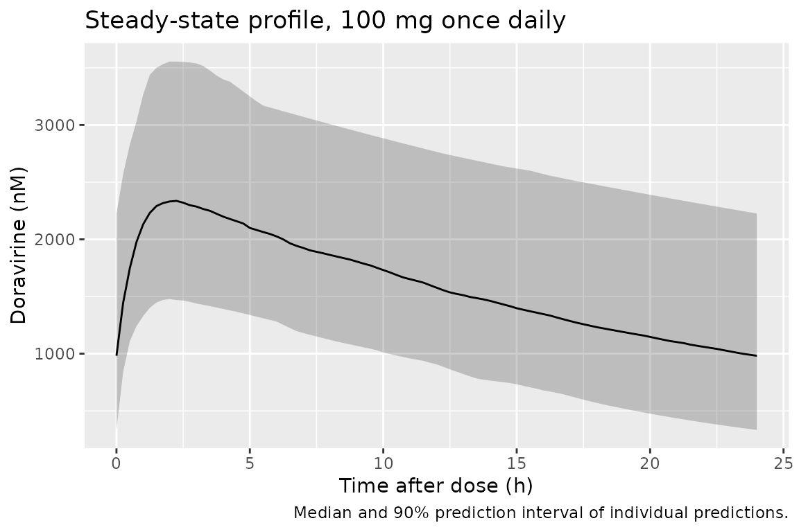
Vaddady 2020 and Yee 2019 publish the centring values of the covariates but not their distributions. The cohort below draws age from a normal distribution centred at 36 years (SD 10, redrawn outside 18-75 years) and weight from a log-normal distribution with median 75 kg (18% CV, redrawn outside 40-150 kg). Everyone is a person living with HIV-1 in a phase 3 study, on 100 mg once daily for 15 days.
set.seed(20201020)
rxode2::rxSetSeed(20201020)

draw_bounded <- function(n, rfun, lo, hi) {
  x <- rfun(n)
  bad <- x < lo | x > hi
  while (any(bad)) {
    x[bad] <- rfun(sum(bad))
    bad <- x < lo | x > hi
  }
  x
}

n_sub <- 200
cov_df <- data.frame(
  id = seq_len(n_sub),
  AGE = draw_bounded(n_sub, function(n) rnorm(n, 36, 10), 18, 75),
  WT = draw_bounded(n_sub, function(n) 75 * exp(rnorm(n, 0, 0.18)), 40, 150)
)

base_ev <- make_ss_events(100, dt = 0.25) |>
  dplyr::select(-id, -AGE, -WT)
events <- cov_df |>
  dplyr::cross_join(base_ev) |>
  dplyr::mutate(treatment = "100 mg QD") |>
  dplyr::arrange(id, time, dplyr::desc(evid))
stopifnot(!anyDuplicated(events[, c("id", "time", "evid")]))
Simulation
sim <- rxode2::rxSolve(mod, events = events, keep = c("treatment")) |>
  as.data.frame()
#> ℹ parameter labels from comments will be replaced by 'label()'
PKNCA validation
The published exposures are steady-state AUC0-24, Cmax and C24 in nM,
so the NCA runs on the last dosing interval (336-360 h) after converting
Cc to nM.
sim_nca <- sim |>
  dplyr::filter(!is.na(Cc)) |>
  dplyr::mutate(Cc = Cc * 1e6 / mw) |>
  dplyr::select(id, time, Cc, treatment)

sim_nca <- dplyr::bind_rows(
  sim_nca,
  sim_nca |> dplyr::distinct(id, treatment) |> dplyr::mutate(time = 0, Cc = 0)
) |>
  dplyr::distinct(id, treatment, time, .keep_all = TRUE) |>
  dplyr::arrange(id, treatment, time)

conc_obj <- PKNCA::PKNCAconc(sim_nca, Cc ~ time | treatment + id)

dose_df <- events |>
  dplyr::filter(evid == 1) |>
  dplyr::select(id, time, amt, treatment)
dose_obj <- PKNCA::PKNCAdose(dose_df, amt ~ time | treatment + id)

# The grid ends exactly at 360 h, so clast.obs is C24.
intervals <- data.frame(
  start = 336, end = 360,
  auclast = TRUE, cmax = TRUE, clast.obs = TRUE
)
nca_res <- PKNCA::pk.nca(PKNCA::PKNCAdata(conc_obj, dose_obj, intervals = intervals))

nca_ind <- as.data.frame(nca_res$result) |>
  dplyr::select(id, treatment, PPTESTCD, PPORRES) |>
  tidyr::pivot_wider(names_from = PPTESTCD, values_from = PPORRES) |>
  dplyr::mutate(auclast = auclast / 1000) # nM h -> uM h
Comparison against published NCA
Vaddady 2020 Table 1 reports geometric means, so the simulated side is aggregated as a geometric mean as well.
geo_mean <- function(x) exp(mean(log(x)))
simulated <- nca_ind |>
  dplyr::group_by(treatment) |>
  dplyr::summarise(
    auclast = geo_mean(auclast),
    cmax = geo_mean(cmax),
    clast.obs = geo_mean(clast.obs),
    .groups = "drop"
  )

published <- tibble::tribble(
  ~treatment, ~auclast, ~cmax, ~clast.obs,
  "100 mg QD", 38.1, 2290, 932
)

cmp <- nlmixr2lib::ncaComparisonTable(
  simulated = simulated,
  reference = published,
  by = "treatment",
  units = c(auclast = "uM*h", cmax = "nM", clast.obs = "nM"),
  tolerance_pct = 20
)
knitr::kable(
  cmp,
  caption = paste(
    "Simulated vs. published (Vaddady 2020 Table 1, treatment-naive phase 3,",
    "N = 730) steady-state geometric means. AUC is AUC0-24 and the last observed concentration (clast.obs, at 24 h post dose) is C24.",
    "* differs from reference by >20%."
  )
)| NCA parameter | treatment | Reference | Simulated | % diff |
|---|---|---|---|---|
| Cmax (nM) | 100 mg QD | 2290 | 2320 | +1.2% |
| Clast (nM) | 100 mg QD | 932 | 935 | +0.3% |
| AUClast (uM*h) | 100 mg QD | 38.1 | 38.5 | +1.1% |
gcv <- function(x) 100 * sqrt(exp(stats::var(log(x))) - 1)
spread <- nca_ind |>
  dplyr::summarise(
    `AUC0-24 geo %CV` = gcv(auclast),
    `Cmax geo %CV` = gcv(cmax),
    `C24 geo %CV` = gcv(clast.obs)
  )
knitr::kable(
  spread,
  digits = 1,
  caption = "Simulated between-subject spread (published treatment-naive: 28.8%, 18.2%, 62.7%)."
)| AUC0-24 geo %CV | Cmax geo %CV | C24 geo %CV |
|---|---|---|
| 35.5 | 26.1 | 67 |
# Structural gate on the centre of the distribution: a mis-transcribed CL/F,
# V/F or dose band moves these by tens of percent.
stopifnot(
  abs(simulated$auclast / 38.1 - 1) < 0.15,
  abs(simulated$cmax / 2290 - 1) < 0.15,
  abs(simulated$clast.obs / 932 - 1) < 0.25
)
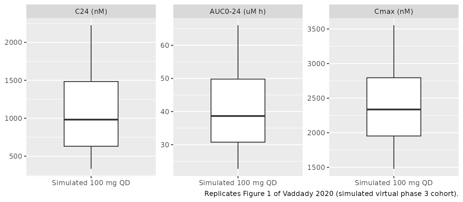
The simulated geometric means agree with the published treatment-naive values. The simulated between-subject spread is somewhat wider than the published one, most visibly for AUC0-24 and Cmax. That is expected: the published values are computed from post hoc (empirical Bayes) parameter estimates, which shrink toward the typical value when the data are sparse (the reported eta-shrinkage on V/F is 43.1%), whereas the simulation draws the full IIV. The DRIVE-SHIFT ISG row of Table 1 (AUC0-24 41.5 uM h, Cmax 2,390 nM, C24 1,110 nM, N = 443) is about 9% higher on AUC; within the model this corresponds to an older cohort (age lowers CL/F by 0.54% per year above 34 years), and the paper concludes the two populations are comparable.
Replicate published figures
# Replicates Figure 1 of Vaddady 2020: distribution of steady-state C24,
# AUC0-24 and Cmax after 100 mg once daily (boxes 25th/50th/75th percentiles,
# whiskers 5th/95th percentiles).
fig1 <- nca_ind |>
  dplyr::transmute(
    `C24 (nM)` = clast.obs,
    `AUC0-24 (uM h)` = auclast,
    `Cmax (nM)` = cmax
  ) |>
  tidyr::pivot_longer(dplyr::everything(), names_to = "metric") |>
  dplyr::group_by(metric) |>
  dplyr::summarise(
    ymin = quantile(value, 0.05), lower = quantile(value, 0.25),
    middle = quantile(value, 0.5), upper = quantile(value, 0.75),
    ymax = quantile(value, 0.95), .groups = "drop"
  ) |>
  dplyr::mutate(metric = factor(metric, levels = c("C24 (nM)", "AUC0-24 (uM h)", "Cmax (nM)")))

ggplot(fig1, aes(x = "Simulated 100 mg QD")) +
  geom_boxplot(
    aes(ymin = ymin, lower = lower, middle = middle, upper = upper, ymax = ymax),
    stat = "identity", width = 0.5
  ) +
  facet_wrap(~metric, scales = "free_y") +
  labs(
    x = NULL, y = NULL,
    caption = "Replicates Figure 1 of Vaddady 2020 (simulated virtual phase 3 cohort)."
  )
sim |>
  dplyr::filter(time >= 336) |>
  dplyr::mutate(tad = time - 336, Cc_nM = Cc * 1e6 / mw) |>
  dplyr::group_by(tad) |>
  dplyr::summarise(
    Q05 = quantile(Cc_nM, 0.05), Q50 = quantile(Cc_nM, 0.5),
    Q95 = quantile(Cc_nM, 0.95), .groups = "drop"
  ) |>
  ggplot(aes(tad, Q50)) +
  geom_ribbon(aes(ymin = Q05, ymax = Q95), alpha = 0.25) +
  geom_line() +
  labs(
    x = "Time after dose (h)", y = "Doravirine (nM)",
    title = "Steady-state profile, 100 mg once daily",
    caption = "Median and 90% prediction interval of individual predictions."
  )
Assumptions and deviations
-
Covariate-equation forms from the predecessor.
Vaddady 2020 prints the age and weight equations but not how the
healthy-versus-HIV-1 status enters V/F. The model uses the Yee 2019
form, `V = TVV * (1 + theta_WT * (WT - 75))
- (1 + theta_healthy * flag)` with flag = 1 for healthy volunteers, since Vaddady 2020 states that the prior model structure was re-estimated unchanged.
-
Residual error. Additive on log-transformed
concentrations (Yee 2019), encoded as
lnorm(). The SDs are selected by study phase (STUDY_PHASE2/STUDY_PHASE3) and, for phase 1, by time after the most recent dose (tad(), 0.5 h cut-off). The table labels are transcribed as printed: 0.224 for phase 1 records at or before 0.5 h postdose and 1.25 after 0.5 h. Both Vaddady 2020 Table S1 and Yee 2019 Table 2 print this assignment, although the Yee 2019 prose (the early-absorption samples being the poorly described ones) reads more naturally with the larger SD on the early records. The choice affects only simulated observation noise, never the individual predictions. -
Dose bands. F1 bands are
< 30 mg,30-120 mgand> 120 mg; a dose of exactly 30 or 120 mg falls in the reference band.DOSE_DORAVIRINE_MGmust be set to the per-administration dose. - No IIV on Ka: none was estimated in either paper.
- Virtual cohort. Age and weight distributions are assumptions centred on the published centring values; the papers do not report the distributions for the combined data set.
- Exposure-response. Not packaged: the paper reports only that the logistic-regression slopes were not significantly different from zero, with no intercept or slope estimates.
- No correction notice was found for Vaddady 2020 (checked 2026-09-27).