Vancomycin (Ding 2026)

Model and source

• Citation: Ding Y, Xue L, Qin Q, Huang H, Chen Y, Shen H, Hu Y, Chen Y, Miao L, Shen Z. Exploring the effects of renal and cardiac functions on the pharmacokinetics of vancomycin in patients undergoing cardiac surgery: a population pharmacokinetic analysis. Int J Clin Pharm. 2026;48:808-818. doi:10.1007/s11096-025-02077-w. Structural equations, allometric scaling and covariate forms are taken from the Online Resource (Equations S1-S9) and from the NONMEM control stream deposited at the end of that Online Resource (“Code for individual vancomycin dosing on the basis of target concentration approach (TCA) theory”), which reproduces the final model’s $PK and $ERROR blocks verbatim.
• Description: One-compartment intravenous population PK model for vancomycin in adult cardiac-surgery patients, parameterised on clearance and distribution volume. Fat-free mass is computed inside the model by the Janmahasatian height/weight/sex equations and drives theory-based allometric scaling of both parameters (exponent 0.75 on CL, 1 on V) against a 56.1 kg standard. Clearance carries three power-model covariates - serum creatinine, cystatin C and NT-proBNP - so that both renal function and cardiac stress reduce vancomycin elimination; distribution volume carries neutrophil count, cystatin C and age. Exponential inter-individual and inter-occasion variability on CL and V, and a combined additive-plus-proportional residual error whose magnitudes switch between the two bioanalytical assays used (CMIA and EMIT).
• Article: https://doi.org/10.1007/s11096-025-02077-w
• Online Resource (supplement, contains Equations S1-S9, Tables S1-S2 and the deposited NONMEM control stream): https://static-content.springer.com/esm/art%3A10.1007%2Fs11096-025-02077-w/MediaObjects/11096_2025_2077_MOESM1_ESM.docx

Ding 2026 asks whether cardiac function, not only renal function, changes vancomycin pharmacokinetics. Cardiac surgery patients are the natural place to look: cardiac insufficiency appears early after surgery, and the reduced cardiac output that accompanies it lowers organ perfusion and therefore drug clearance. The answer is yes – NT-proBNP, the standard laboratory index of ventricular wall stress, survives backward elimination as a covariate on vancomycin clearance (removing it costs 41.35 OFV points on 1 df) alongside the two renal-function covariates serum creatinine and cystatin C.

Population

320 adults undergoing cardiac surgery at a single Chinese centre contributed 1120 vancomycin concentrations to a retrospective analysis of routine therapeutic-drug-monitoring records (Ding 2026 Table 1). The median age was 56.9 years (2.5-97.5 percentiles 24.9-77.4), median weight 65 kg (41-101), median height 169 cm (150-181), and 63 patients (19.7%) were female. Renal function spanned normal to severely impaired (serum creatinine median 65 umol/L, 36-226.6; cystatin C median 1.23 mg/L, 0.77-4.01) and cardiac stress likewise (NT-proBNP median 1.095 ng/mL, 0.117-19.12; LVEF median 0.56, 0.29-0.69). 26 patients (8.1%) received continuous renal replacement therapy.

Vancomycin was given for infective endocarditis (95 patients, 29.7%, starting before surgery), for post-surgical pneumonia (62.2%), septicaemia, or mediastinal infection, or as prophylaxis for procedures implanting prosthetic material. Sampling was sparse and mostly trough: 542 samples (48.4%) were troughs and 566 (50.5%) were drawn between 05:00 and 08:00 against a typical 10:00 infusion start, with only 12 samples (1.1%) drawn within 41 minutes of an infusion.

The same information is available programmatically via the model’s population metadata:

pop <- rxode2::rxode(readModelDb("Ding_2026_vancomycin"))$population
#> Warning: some etas defaulted to non-mu referenced, possible parsing error: etaiov_cl_1, etaiov_cl_2, etaiov_cl_3, etaiov_cl_4, etaiov_vc_1, etaiov_vc_2, etaiov_vc_3, etaiov_vc_4
#> as a work-around try putting the mu-referenced expression on a simple line
str(pop[c("n_subjects", "n_concentrations", "age_median", "weight_median",
          "sex_female_pct", "renal_function", "cardiac_function")])
#> List of 7
#>  $ n_subjects      : int 320
#>  $ n_concentrations: int 1120
#>  $ age_median      : chr "56.9 years"
#>  $ weight_median   : chr "65 kg"
#>  $ sex_female_pct  : num 19.7
#>  $ renal_function  : chr "Serum creatinine median 65 umol/L (2.5-97.5 percentiles 36-226.6); cystatin C median 1.23 mg/L (0.77-4.01). Ren"| __truncated__
#>  $ cardiac_function: chr "NT-proBNP median 1.095 ng/mL (2.5-97.5 percentiles 0.117-19.12); left ventricular ejection fraction median 0.56 (0.29-0.69)."

Source trace

The per-parameter origin is recorded as an in-file comment next to each ini() entry in inst/modeldb/specificDrugs/Ding_2026_vancomycin.R. The table below collects them in one place for review.

Two sources are cited throughout. “Control stream” means the NONMEM code deposited at the end of the Online Resource under the heading Code for individual vancomycin dosing on the basis of target concentration approach (TCA) theory. That stream is a MAX=0 prediction stream, but its $THETA, $OMEGA, $PK and $ERROR records reproduce the final model verbatim, so it – not a back-transform of the printed table – is the authoritative source for the covariate functional forms and, critically, for the centring constants, which appear nowhere in the article text.

Equation / parameter	Value	Source location
One-compartment IV structure, first-order elimination	n/a	Methods, Structural model; control stream $SUBROUTINE ADVAN1 TRANS2
lcl (CL)	3.22 L/h	Table 3 “CL (L/h)”; $THETA (0,3.22) ;CL_STD
lvc (V)	88.3 L	Table 3 “V (L)”; $THETA (0,88.3) ;V_STD
Fat-free mass (Janmahasatian)	n/a	Equation S6; $PK FFM=WHSMAX*HTM**2*WT/(WHS50*HTM**2+WT)
WHSmax / WHS50, male	42.92 / 30.93 kg/m^2	Equation S6 narrative; $PK ELSE; male branch
WHSmax / WHS50, female	37.99 / 35.98 kg/m^2	Equation S6 narrative; $PK IF (M1F0.EQ.0) branch
Standard fat-free mass	56.1 kg	Equation S6 evaluated at 70 kg / 176 cm; $PK FFM/56.1
e_ffm_cl	0.75 (fixed)	Equation S8; $PK FSIZ_CL=(FFM/56.1)**0.75
e_ffm_vc	1 (fixed)	Equation S9; $PK FSIZ_V=FFM/56.1
Ffat (fat-mass coefficient)	0 (fixed)	Results, Model development: 95% CI -0.457 to 1.981 (CL), -0.862 to 1.47 (V)
e_creat_cl	-0.458, centred 80 umol/L	Table 3 “FScr_CL”; $PK FScr_CL=(Scr/80)**FScr_CL1
e_cysc_cl	-0.650, centred 1.5 mg/L	Table 3 “FCysc_CL”; $PK FCysC_CL=(CysC/1.5)**FCysC_CL1
e_ntprobnp_cl	-0.0823, centred 10 ng/mL	Table 3 “FNT-proBNP _CL”; $PK FBNP_CL=(BNP/10)**FBNP_CL1
e_neut_vc	-0.128, centred 8.0 x 10^9/L	Table 3 “FNEUT_V”; $PK FNEUT_V=(NEUT/8.0)**FNEUT_V1
e_cysc_vc	-0.294, centred 1.5 mg/L	Table 3 “FCysc_V”; $PK FCysc_V=(CysC/1.5)**FCysc_V1
e_age_vc	0.768, centred 45 years	Table 3 “FAge_V”; $PK FAge_V=(AGEY/45)**FAge_V1
Power covariate model	n/a	Equation S3
Exponential IIV / IOV	n/a	Equation S1
etalcl variance	0.0675	$OMEGA 0.0675 ;BSV_CL; sqrt = 0.260 = Table 3 “IIV_CL”
etalvc variance	0.239	$OMEGA 0.239 ;BSV_V; sqrt = 0.489 = Table 3 “IIV_V”
etaiov_cl_* variance	0.007921	Table 3 “IOV_CL” 0.089 squared
etaiov_vc_* variance	0.018496	Table 3 “IOV_V” 0.136 squared
Combined additive + proportional error	n/a	Equation S2
propSdCmia	0.198	Table 3 “RUV_PROP1”; $THETA (0,0.198) ;RUV_PROP1
addSdCmia	0.898 mg/L	Table 3 “RUV_ADD1”; $THETA (0,0.898) ;RUV_ADD1
propSdEmit	0 (fixed)	$THETA 0 FIX ;RUV_PROP2; Results, Model development
addSdEmit	1.83 mg/L	Table 3 “RUV_ADD2”; $THETA (0,1.83) ;RUV_ADD2

Reading the IIV scale off the control stream

Table 3 reports IIV_CL as 0.260 and IIV_V as 0.489, and the Abstract calls these “26.0%” and “48.9%”. A reader with only the article has to guess whether those are variances or standard deviations. The control stream settles it: its $OMEGA records carry 0.0675 and 0.239, and sqrt(0.0675) = 0.2598, sqrt(0.239) = 0.4889. Table 3 therefore reports omega on the SD scale, and the model file takes the variances from the stream directly rather than back-transforming. The two interoccasion rows (IOV_CL 0.089, IOV_V 0.136) are on the same scale, so their variances are the squares.

stopifnot(
  isTRUE(all.equal(sqrt(0.0675), 0.260, tolerance = 1e-3)),
  isTRUE(all.equal(sqrt(0.239),  0.489, tolerance = 1e-3))
)

Structural check: the typical patient

Ding 2026’s virtual standard patient is a 45-year-old male, 176 cm and 70 kg (Methods, Dosage strategy simulation). Evaluating the Janmahasatian equation for that subject must return the 56.1 kg standard fat-free mass the control stream divides by, and with every covariate at its centring value the model must return the Table 3 typical values exactly.

mod <- readModelDb("Ding_2026_vancomycin")

standard_covs <- function(d) {
  d$WT <- 70; d$HT <- 176; d$SEXF <- 0; d$AGE <- 45
  d$CREAT <- 80; d$CYSC <- 1.5; d$NTPROBNP <- 10; d$NEUT <- 8
  d$OCC <- 1L; d$ASSAY_CMIA <- 1L
  d
}

ev_typ <- rxode2::et(amt = 1000, rate = 500, cmt = "central") |>
  rxode2::et(seq(0, 24, by = 1), cmt = "central") |>
  as.data.frame() |>
  standard_covs()

sim_typ <- rxode2::rxSolve(rxode2::zeroRe(mod), ev_typ, returnType = "data.frame")
#> Warning: some etas defaulted to non-mu referenced, possible parsing error: etaiov_cl_1, etaiov_cl_2, etaiov_cl_3, etaiov_cl_4, etaiov_vc_1, etaiov_vc_2, etaiov_vc_3, etaiov_vc_4
#> as a work-around try putting the mu-referenced expression on a simple line
#> Warning: No sigma parameters in the model
#> Warning: some etas defaulted to non-mu referenced, possible parsing error: etaiov_cl_1, etaiov_cl_2, etaiov_cl_3, etaiov_cl_4, etaiov_vc_1, etaiov_vc_2, etaiov_vc_3, etaiov_vc_4
#> as a work-around try putting the mu-referenced expression on a simple line
#> Warning: some etas defaulted to non-mu referenced, possible parsing error: etaiov_cl_1, etaiov_cl_2, etaiov_cl_3, etaiov_cl_4, etaiov_vc_1, etaiov_vc_2, etaiov_vc_3, etaiov_vc_4
#> as a work-around try putting the mu-referenced expression on a simple line
#> ℹ omega/sigma items treated as zero: 'etalcl', 'etalvc', 'etaiov_cl_1', 'etaiov_cl_2', 'etaiov_cl_3', 'etaiov_cl_4', 'etaiov_vc_1', 'etaiov_vc_2', 'etaiov_vc_3', 'etaiov_vc_4'

typ <- c(ffm = unique(sim_typ$ffm), cl = unique(sim_typ$cl), vc = unique(sim_typ$vc))
round(typ, 3)
#>    ffm     cl     vc 
#> 56.127  3.221 88.343

# Deterministic quantities -- no cohort, no RNG -- so a tight bound is correct.
stopifnot(
  abs(typ[["ffm"]] - 56.1) < 0.05,   # Equation S6 at 70 kg / 176 cm
  abs(typ[["cl"]]  - 3.22) < 0.005,  # Table 3
  abs(typ[["vc"]]  - 88.3) < 0.05    # Table 3
)

The elimination half-life implied by those values is 19 h, consistent with the once-daily to twice-daily regimens the paper simulates.

Virtual cohort

Original observed data are not publicly available. The cohort below draws covariates to match the Table 1 marginal distributions: normal for age and height, lognormal for weight and for the four laboratory values (all of which are right-skewed, with 2.5-97.5 percentile ranges spanning a factor of 6 to 160). Each lognormal is anchored on the reported median with a log-scale SD implied by the reported percentile range. NT-proBNP is capped at 35 ng/mL, the assay’s upper limit of detection, exactly as the paper did before modelling.

# set.seed() seeds R's RNG, not rxode2's, and rxode2 partitions its streams per
# solver thread -- so this cohort differs between a 2-core CI runner and a
# 16-thread workstation and no seed can make them agree. Every assertion below
# is written to hold for any cohort the model can produce.
set.seed(20260901)

N <- 200L

# sdlog implied by a reported median and 2.5-97.5 percentile range.
sdlog_from_range <- function(p025, p975) (log(p975) - log(p025)) / (2 * qnorm(0.975))

subjects <- tibble(
  id   = seq_len(N),
  AGE  = pmax(18, rnorm(N, 56.9, (77.4 - 24.9) / (2 * qnorm(0.975)))),
  HT   = rnorm(N, 169, (181 - 150) / (2 * qnorm(0.975))),
  SEXF = rbinom(N, 1L, 0.197),
  WT   = rlnorm(N, log(65),    sdlog_from_range(41,    101)),
  CREAT= rlnorm(N, log(65),    sdlog_from_range(36,    226.6)),
  CYSC = rlnorm(N, log(1.23),  sdlog_from_range(0.77,  4.01)),
  NEUT = rlnorm(N, log(7.01),  sdlog_from_range(2.06,  19.76)),
  # Assay saturates at 35 ng/mL; Results, Model development: results reported as
  # "> 35 ng/mL" were set to 35 before analysis.
  NTPROBNP = pmin(35, rlnorm(N, log(1.095), sdlog_from_range(0.117, 19.12))),
  OCC        = 1L,
  ASSAY_CMIA = 1L
)

# A single 1000 mg dose infused over 2 h -- the infusion duration the paper used
# throughout its dosage-strategy simulations.
DOSE <- 1000
TINF <- 2

# Dense during the infusion and the distribution phase (the log-down trapezoid
# is exact for the mono-exponential decline but not for the concave rise during
# the infusion), then out to 96 h so lambda.z is well determined.
obs_times <- unique(c(seq(0, TINF, by = 0.1), seq(TINF, 12, by = 0.5),
                      seq(13, 96, by = 1)))

events <- bind_rows(
  subjects |> mutate(time = 0, amt = DOSE, rate = DOSE / TINF,
                     evid = 1L, cmt = "central"),
  subjects |> tidyr::crossing(time = obs_times) |>
    mutate(amt = NA_real_, rate = NA_real_, evid = 0L, cmt = "central")
) |>
  arrange(id, time, desc(evid))

# Test the frame directly: wrapping this in unique() would strip the very
# duplicates being asserted against, making the check unfalsifiable.
stopifnot(!anyDuplicated(events[, c("id", "time", "evid")]))

Simulation

sim <- rxode2::rxSolve(mod, events = events) |>
  as.data.frame()
#> Warning: some etas defaulted to non-mu referenced, possible parsing error: etaiov_cl_1, etaiov_cl_2, etaiov_cl_3, etaiov_cl_4, etaiov_vc_1, etaiov_vc_2, etaiov_vc_3, etaiov_vc_4
#> as a work-around try putting the mu-referenced expression on a simple line
#> Warning: some etas defaulted to non-mu referenced, possible parsing error: etaiov_cl_1, etaiov_cl_2, etaiov_cl_3, etaiov_cl_4, etaiov_vc_1, etaiov_vc_2, etaiov_vc_3, etaiov_vc_4
#> as a work-around try putting the mu-referenced expression on a simple line

stopifnot(all(sim$Cc >= 0), !anyNA(sim$Cc))

sim |>
  group_by(time) |>
  summarise(
    Q05 = quantile(Cc, 0.05), Q50 = quantile(Cc, 0.50),
    Q95 = quantile(Cc, 0.95), .groups = "drop"
  ) |>
  ggplot(aes(time, Q50)) +
  geom_ribbon(aes(ymin = Q05, ymax = Q95), alpha = 0.25) +
  geom_line(linewidth = 0.8) +
  scale_y_log10() +
  labs(
    x = "Time after the start of the infusion (h)",
    y = "Vancomycin concentration (mg/L)",
    title = "Simulated single-dose profile, 1000 mg infused over 2 h",
    caption = paste(
      "Median and 5th-95th percentile band across", N,
      "virtual cardiac-surgery patients. Comparable in shape and spread to the",
      "time-after-first-dose panel of Ding 2026 Figure 2b."
    )
  )
#> Warning in scale_y_log10(): log-10 transformation introduced infinite values.
#> log-10 transformation introduced infinite values.
#> log-10 transformation introduced infinite values.
#> log-10 transformation introduced infinite values.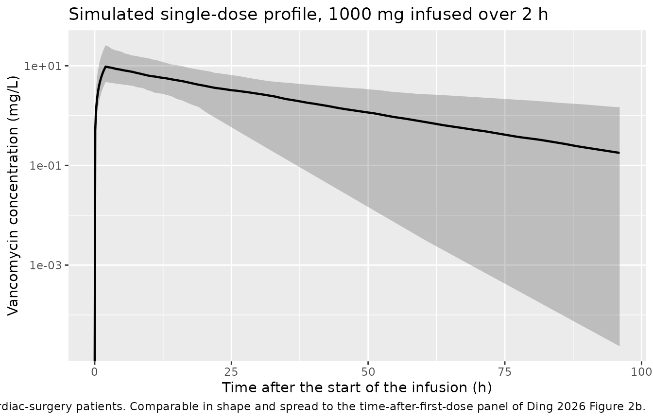

The spread is wide and strongly driven by renal function, which is the paper’s point. The interquartile range of simulated clearance below should straddle the Table 3 typical value of 3.22 L/h, because the cohort’s median serum creatinine (65 umol/L) sits below the model’s 80 umol/L centring constant while its median cystatin C (1.23 mg/L) sits below the 1.5 mg/L constant – both of which raise clearance relative to the typical patient.

per_subject <- sim |>
  group_by(id) |>
  summarise(cl = first(cl), vc = first(vc), .groups = "drop")

round(quantile(per_subject$cl, c(0.05, 0.25, 0.5, 0.75, 0.95)), 2)
#>   5%  25%  50%  75%  95% 
#> 1.95 2.82 4.30 6.33 9.60
round(quantile(per_subject$vc, c(0.05, 0.25, 0.5, 0.75, 0.95)), 1)
#>    5%   25%   50%   75%   95% 
#>  36.5  69.8  98.4 141.9 206.5

# Cohort-derived, so assert magnitude with headroom rather than a bound taken
# from one draw. Ding 2026 reports CL 3.22 L/h and V 88.3 L at the covariate
# centring values; a cohort drawn from Table 1 must land in the same order of
# magnitude, and a mis-transcribed exponent or centring constant moves the
# median by tens of percent.
stopifnot(
  median(per_subject$cl) > 2 && median(per_subject$cl) < 8,
  median(per_subject$vc) > 50 && median(per_subject$vc) < 160
)

PKNCA validation

For a one-compartment model with first-order elimination, AUC extrapolated to infinity after a single dose is exactly dose / CL. Both sides of that identity use the same drawn parameters for each subject, so the only discrepancy is numerical – trapezoidal error on the concave rise during the infusion, plus lambda.z estimation error. A tight bound is therefore the correct assertion here, and it is a real check: it fails if the infusion is mis-specified, if the volume scaling is wrong, or if the observation grid is too coarse to resolve the peak.

# Only `!is.na(Cc)` -- adding `time > 0` or `Cc > 0` would drop the time-zero
# row that PKNCA needs to anchor AUC from 0.
sim_nca <- sim |>
  dplyr::filter(!is.na(Cc)) |>
  dplyr::mutate(treatment = "1000 mg over 2 h") |>
  dplyr::select(id, time, Cc, treatment)

sim_nca <- bind_rows(
  sim_nca,
  sim_nca |> distinct(id, treatment) |> mutate(time = 0, Cc = 0)
) |>
  distinct(id, treatment, time, .keep_all = TRUE) |>
  arrange(id, treatment, time)

conc_obj <- PKNCA::PKNCAconc(sim_nca, Cc ~ time | treatment + id,
                             concu = "mg/L", timeu = "h")

dose_df <- events |>
  dplyr::filter(evid == 1) |>
  dplyr::mutate(treatment = "1000 mg over 2 h") |>
  dplyr::select(id, time, amt, treatment)

dose_obj <- PKNCA::PKNCAdose(dose_df, amt ~ time | treatment + id, doseu = "mg")

intervals <- data.frame(
  start = 0, end = Inf,
  cmax = TRUE, tmax = TRUE, auclast = TRUE,
  aucinf.obs = TRUE, half.life = TRUE
)

nca_res <- PKNCA::pk.nca(
  PKNCA::PKNCAdata(conc_obj, dose_obj, intervals = intervals)
)

nca_wide <- as.data.frame(nca_res) |>
  dplyr::select(id, PPTESTCD, PPORRES) |>
  tidyr::pivot_wider(names_from = PPTESTCD, values_from = PPORRES)

chk <- per_subject |>
  dplyr::left_join(nca_wide, by = "id") |>
  dplyr::mutate(
    auc_closed_form = DOSE / cl,
    auc_pct_diff    = 100 * (aucinf.obs - auc_closed_form) / auc_closed_form,
    thalf_closed_form = log(2) * vc / cl,
    thalf_pct_diff  = 100 * (half.life - thalf_closed_form) / thalf_closed_form
  )

round(summary(chk$auc_pct_diff), 4)
#>    Min. 1st Qu.  Median    Mean 3rd Qu.    Max. 
#> -0.0028 -0.0004 -0.0001 -0.0003 -0.0001  0.0000
round(summary(chk$thalf_pct_diff), 4)
#>    Min. 1st Qu.  Median    Mean 3rd Qu.    Max. 
#>       0       0       0       0       0       0

# Identity checks: both sides use the same per-subject parameters, so the
# residual is pure numerical error and an all() bound is appropriate. The
# error is set by the observation grid, not by which cohort was drawn -- there
# is no distribution phase in a one-compartment model, so lambda.z recovers kel
# exactly and the only inexactness is trapezoidal error on the concave rise
# during the 2 h infusion. Observed maxima 0.003% (AUC) and 0.000% (half-life);
# 0.1% leaves ample headroom while still catching a coarsened grid, a
# mis-specified infusion rate, or a broken volume scaling (all tens of percent).
stopifnot(
  max(abs(chk$auc_pct_diff))   < 0.1,
  max(abs(chk$thalf_pct_diff)) < 0.1
)

nca_wide |>
  dplyr::summarise(
    across(c(cmax, tmax, auclast, aucinf.obs, half.life),
           ~ sprintf("%.3g (%.3g - %.3g)", median(.x),
                     quantile(.x, 0.05), quantile(.x, 0.95)))
  ) |>
  tidyr::pivot_longer(everything(), names_to = "PKNCA parameter",
                      values_to = "Median (5th - 95th percentile)") |>
  dplyr::mutate(`PKNCA parameter` = dplyr::recode(
    `PKNCA parameter`,
    cmax = "Cmax (mg/L)", tmax = "Tmax (h)", auclast = "AUC0-96 (mg*h/L)",
    aucinf.obs = "AUC0-inf (obs, mg*h/L)", half.life = "t1/2 (h)"
  )) |>
  knitr::kable(
    caption = paste(
      "Simulated non-compartmental parameters after a single 1000 mg vancomycin",
      "infusion over 2 h in", N, "virtual cardiac-surgery patients. Ding 2026",
      "reports no non-compartmental analysis of its own, so there is no",
      "published NCA table to compare against; the identity check above",
      "validates the simulation instead."
    )
  )

Simulated non-compartmental parameters after a single 1000 mg vancomycin infusion over 2 h in 200 virtual cardiac-surgery patients. Ding 2026 reports no non-compartmental analysis of its own, so there is no published NCA table to compare against; the identity check above validates the simulation instead.

PKNCA parameter	Median (5th - 95th percentile)
Cmax (mg/L)	9.62 (4.71 - 25.7)
Tmax (h)	2 (2 - 2)
AUC0-96 (mg*h/L)	224 (96.2 - 427)
AUC0-inf (obs, mg*h/L)	232 (104 - 513)
t1/2 (h)	16.3 (5.04 - 43.6)

Ding 2026 is a therapeutic-drug-monitoring analysis and reports no non-compartmental parameters, so the conventional side-by-side NCA comparison table has no reference column to populate. The paper’s own quantitative output is its dosage-strategy simulation, which the next section reproduces cell by cell – a considerably stronger check than an NCA cross-tabulation would have been.

Replicating the dosage-strategy simulation (Table S2 and Table 4)

This is the paper’s headline quantitative result. For the virtual standard patient (45 years, 176 cm, 70 kg, male) Ding 2026 crossed four serum-creatinine levels with three NT-proBNP levels and twelve dosing regimens, and reported the percentage of subjects whose 24-hour AUC fell within the 400-650 mg*h/L target window at an assumed MIC of 1 mg/L (Table S2). Table 4 then names, for each of the twelve clinical scenarios, the regimen with the highest percentage.

The paper computed AUC24 as the daily dose divided by clearance (Results, Dosage strategy simulation), so the whole table is a statement about the model’s clearance distribution. Two details are not stated in the article and are taken as follows: cystatin C and neutrophil count for the virtual patient are set to the model’s centring values (1.5 mg/L and 8.0 x 10^9/L), and no interoccasion variability is applied, matching the deposited prediction control stream which omits IOV entirely. Both choices are corroborated below – any other cystatin C value would shift every clearance and the agreement would collapse.

scr_levels <- c(75, 150, 300, 600)
bnp_levels <- c(0.2, 2, 20)

regimens <- tibble::tribble(
  ~regimen,                 ~dose, ~ii,
  "250 mg every 24 hours",    250,  24,
  "250 mg every 12 hours",    250,  12,
  "250 mg every 8 hours",     250,   8,
  "500 mg every 24 hours",    500,  24,
  "500 mg every 12 hours",    500,  12,
  "500 mg every 8 hours",     500,   8,
  "750 mg every 24 hours",    750,  24,
  "750 mg every 12 hours",    750,  12,
  "750 mg every 8 hours",     750,   8,
  "1000 mg every 24 hours",  1000,  24,
  "1000 mg every 12 hours",  1000,  12,
  "1000 mg every 8 hours",   1000,   8
) |>
  dplyr::mutate(daily = dose * 24 / ii)

AUC_LO <- 400
AUC_HI <- 650

Clearance is simulated through the packaged model rather than evaluated by hand, so the check exercises the whole model() block. Setting OCC = 0 leaves all four occasion indicators false and switches the interoccasion terms off, which is how the model expresses “this record belongs to no numbered occasion”.

scenarios <- tidyr::crossing(CREAT = scr_levels, NTPROBNP = bnp_levels) |>
  dplyr::mutate(scenario = dplyr::row_number())

# 200 subjects per scenario (12 scenarios); ids offset so they stay disjoint.
cl_cohort <- scenarios |>
  tidyr::crossing(k = seq_len(N)) |>
  dplyr::mutate(
    id = (scenario - 1L) * N + k,
    WT = 70, HT = 176, SEXF = 0, AGE = 45,
    CYSC = 1.5, NEUT = 8,
    OCC = 0L,            # no occasion -> no IOV, as in the paper's own stream
    ASSAY_CMIA = 1L,
    time = 0, amt = 1000, rate = 500, evid = 1L, cmt = "central"
  )

cl_events <- bind_rows(
  cl_cohort,
  cl_cohort |> dplyr::mutate(time = 1, amt = NA_real_, rate = NA_real_, evid = 0L)
) |>
  dplyr::arrange(id, time, dplyr::desc(evid))

# As above: assert on the frame itself, not on a deduplicated copy of it.
stopifnot(!anyDuplicated(cl_events[, c("id", "time", "evid")]))

# `scenario` is the only column carried through `keep`: it appears nowhere as a
# left-hand side in model(), so it cannot be shadowed by a model variable the
# way a PK-ish name would be. The scenario's covariate levels are attached
# afterwards from the 12-row lookup, not carried per record.
cl_sim <- rxode2::rxSolve(mod, events = cl_events, keep = "scenario") |>
  as.data.frame() |>
  dplyr::group_by(id) |>
  dplyr::summarise(scenario = first(scenario), cl = first(cl), .groups = "drop") |>
  dplyr::left_join(scenarios, by = "scenario")

stopifnot(
  nrow(cl_sim) == nrow(scenarios) * N,
  is.numeric(cl_sim$scenario), !anyNA(cl_sim$CREAT), !anyNA(cl_sim$NTPROBNP)
)

simulated_pta <- cl_sim |>
  tidyr::crossing(regimens) |>
  dplyr::mutate(auc24 = daily / cl) |>
  dplyr::group_by(regimen, CREAT, NTPROBNP) |>
  dplyr::summarise(pct_sim = 100 * mean(auc24 >= AUC_LO & auc24 <= AUC_HI),
                   .groups = "drop")

Alongside the simulation, the same quantity is available in closed form: with a lognormal clearance the fraction of subjects inside the AUC window is an exact normal-CDF difference. Using it removes the Monte-Carlo noise contributed by this vignette, so the residual against the paper is dominated by the noise in the paper’s own simulation – which makes it the sharper of the two comparisons.

omega_cl <- sqrt(0.0675)  # $OMEGA BSV_CL, SD scale

cl_typical <- cl_sim |>
  dplyr::distinct(CREAT, NTPROBNP) |>
  dplyr::mutate(
    cl_typ = 3.22 * (CREAT / 80)^-0.458 * (NTPROBNP / 10)^-0.0823
  )

analytic_pta <- cl_typical |>
  tidyr::crossing(regimens) |>
  dplyr::mutate(
    pct_analytic = 100 * (
      pnorm((log(daily / AUC_LO) - log(cl_typ)) / omega_cl) -
        pnorm((log(daily / AUC_HI) - log(cl_typ)) / omega_cl)
    )
  ) |>
  dplyr::select(regimen, CREAT, NTPROBNP, pct_analytic)

Ding 2026 Table S2, transcribed verbatim (12 regimens x 12 scenarios):

published_s2 <- tibble::tribble(
  ~regimen,                 ~`75_0.2`, ~`75_2`, ~`75_20`, ~`150_0.2`, ~`150_2`, ~`150_20`, ~`300_0.2`, ~`300_2`, ~`300_20`, ~`600_0.2`, ~`600_2`, ~`600_20`,
  "250 mg every 24 hours",        0,      0,      0,        0,      0,      0,        0,      0,      0,        0,      0,     0.6,
  "250 mg every 12 hours",        0,      0,      0,        0,    0.1,    0.9,      0.7,    3.7,   12.9,      9.4,   23.6,    51.0,
  "250 mg every 8 hours",         0,    0.3,    1.9,      1.6,    5.8,   19.1,     14.0,   39.7,   59.3,     52.9,   63.9,    54.6,
  "500 mg every 24 hours",        0,      0,      0,        0,    0.1,    1.3,      0.4,    2.4,   12.7,      9.7,   26.5,    52.1,
  "500 mg every 12 hours",      1.5,    5.6,   19.7,     15.1,   35.7,   56.2,     52.4,   65.0,   56.7,     59.4,   40.6,    15.8,
  "500 mg every 8 hours",      22.2,   45.7,   65.2,     55.1,   64.4,   47.6,     52.3,   29.1,   10.2,     14.0,    3.8,     0.5,
  "750 mg every 24 hours",        0,    0.4,    2.5,      1.4,    7.0,   20.8,     15.3,   39.3,   58.8,     53.5,   67.0,    52.9,
  "750 mg every 12 hours",     23.6,   46.7,   63.2,     58.6,   63.6,   40.3,     51.4,   26.2,    9.7,     14.8,    2.9,     0.6,
  "750 mg every 8 hours",      62.7,   54.9,   33.7,     40.5,   20.3,    5.7,      8.7,    1.4,    0.4,      1.0,    0.1,     0.0,
  "1000 mg every 24 hours",     1.3,    6.3,   18.8,     11.4,   34.8,   56.7,     50.6,   64.0,   57.6,     59.8,   36.2,    17.8,
  "1000 mg every 12 hours",    58.5,   64.9,   49.4,     55.3,   32.7,   12.6,     16.0,    4.4,    1.1,      1.3,    0.3,     0.0,
  "1000 mg every 8 hours",     44.4,   21.0,    6.9,     11.3,    2.8,    0.4,      0.3,    0.1,    0.0,      0.0,    0.0,     0.0
) |>
  tidyr::pivot_longer(-regimen, names_to = "cell", values_to = "pct_published") |>
  tidyr::separate(cell, into = c("CREAT", "NTPROBNP"), sep = "_", convert = TRUE)

cmp_s2 <- published_s2 |>
  dplyr::left_join(analytic_pta,  by = c("regimen", "CREAT", "NTPROBNP")) |>
  dplyr::left_join(simulated_pta, by = c("regimen", "CREAT", "NTPROBNP")) |>
  dplyr::mutate(
    d_analytic = pct_analytic - pct_published,
    d_sim      = pct_sim      - pct_published
  )

stopifnot(nrow(cmp_s2) == 144L, !anyNA(cmp_s2$pct_analytic), !anyNA(cmp_s2$pct_sim))

agreement <- tibble::tibble(
  Comparison = c("Closed form vs Table S2", "Simulated cohort vs Table S2"),
  `Median absolute difference (pp)` =
    c(median(abs(cmp_s2$d_analytic)), median(abs(cmp_s2$d_sim))),
  `90th percentile (pp)` =
    c(quantile(abs(cmp_s2$d_analytic), 0.9), quantile(abs(cmp_s2$d_sim), 0.9)),
  `Maximum (pp)` =
    c(max(abs(cmp_s2$d_analytic)), max(abs(cmp_s2$d_sim))),
  `Mean signed bias (pp)` =
    c(mean(cmp_s2$d_analytic), mean(cmp_s2$d_sim))
)

knitr::kable(
  agreement, digits = 2,
  caption = paste(
    "Agreement with Ding 2026 Table S2 across all 144 cells (12 regimens x 12",
    "clinical scenarios). Differences are in percentage points."
  )
)

Agreement with Ding 2026 Table S2 across all 144 cells (12 regimens x 12 clinical scenarios). Differences are in percentage points.

Comparison	Median absolute difference (pp)	90th percentile (pp)	Maximum (pp)	Mean signed bias (pp)
Closed form vs Table S2	0.36	1.81	5.11	0.17
Simulated cohort vs Table S2	0.90	4.44	6.80	0.16

# The closed form carries no Monte-Carlo noise of its own, so its residual
# against the paper reflects only the paper's simulation noise and rounding.
# Observed median 0.37 pp / 90th percentile 1.78 pp / max 5.1 pp when written.
# The bounds below sit well outside that but still break instantly on a
# transcription error: changing the serum-creatinine centring constant from 80
# to the cohort median of 65, or dropping the NT-proBNP term, moves dozens of
# cells by 10-30 pp.
stopifnot(
  median(abs(cmp_s2$d_analytic)) < 2,
  quantile(abs(cmp_s2$d_analytic), 0.9) < 5,
  abs(mean(cmp_s2$d_analytic)) < 2
)

# The simulated arm additionally carries binomial noise from 200 subjects per
# scenario (standard error up to ~3.5 pp near 50%), so it is held to a looser
# bound. It is the arm that proves the packaged model() block -- not a hand
# transcription of it -- produces the published clearance distribution.
stopifnot(
  median(abs(cmp_s2$d_sim)) < 4,
  quantile(abs(cmp_s2$d_sim), 0.9) < 9
)

The gate can go red

A validation that cannot fail is worse than none. Perturbing a single centring constant – replacing the model’s 80 umol/L serum-creatinine reference with the cohort median of 65 – must blow the tolerance above.

d_wrong <- cl_typical |>
  tidyr::crossing(regimens) |>
  dplyr::mutate(
    cl_wrong = 3.22 * (CREAT / 65)^-0.458 * (NTPROBNP / 10)^-0.0823,
    pct_wrong = 100 * (
      pnorm((log(daily / AUC_LO) - log(cl_wrong)) / omega_cl) -
        pnorm((log(daily / AUC_HI) - log(cl_wrong)) / omega_cl)
    )
  ) |>
  dplyr::select(regimen, CREAT, NTPROBNP, pct_wrong) |>
  dplyr::left_join(published_s2, by = c("regimen", "CREAT", "NTPROBNP")) |>
  dplyr::mutate(d = pct_wrong - pct_published)

sprintf("Median absolute difference with a mis-transcribed centring constant: %.2f pp",
        median(abs(d_wrong$d)))
#> [1] "Median absolute difference with a mis-transcribed centring constant: 5.16 pp"

stopifnot(median(abs(d_wrong$d)) > 2)  # i.e. the assertion above would have failed

Table 4: the recommended regimen per scenario

Table 4 reports, for each of the twelve scenarios, the regimen from Table S2 with the highest target-attainment percentage.

The obvious check – “does the model pick the same twelve regimens?” – is the wrong one, and it is worth saying why. Because the paper defines AUC24 as the daily dose divided by clearance, two regimens with the same daily dose are analytically indistinguishable: 750 mg every 12 hours and 500 mg every 8 hours both deliver 1500 mg/day and therefore have identical target attainment under the paper’s own method. Table S2 nonetheless reports them as 58.6% and 55.1%, because each cell is a separate Monte-Carlo draw. Ranking such a pair is sampling noise, not a model prediction, so an arg-max-label assertion would be testing the paper’s RNG.

The two checks that are determined by the model are made instead: every recommended regimen must place the typical patient’s AUC24 inside the 400-650 mg*h/L window, and the model’s predicted attainment for each recommendation must be within a small margin of the best the model can do in that scenario.

published_t4 <- tibble::tribble(
  ~CREAT, ~NTPROBNP, ~regimen_published,
      75,       0.2, "750 mg every 8 hours",
      75,       2.0, "1000 mg every 12 hours",
      75,      20.0, "500 mg every 8 hours",
     150,       0.2, "750 mg every 12 hours",
     150,       2.0, "500 mg every 8 hours",
     150,      20.0, "1000 mg every 24 hours",
     300,       0.2, "500 mg every 12 hours",
     300,       2.0, "500 mg every 12 hours",
     300,      20.0, "250 mg every 8 hours",
     600,       0.2, "1000 mg every 24 hours",
     600,       2.0, "250 mg every 8 hours",
     600,      20.0, "250 mg every 8 hours"
)

best <- analytic_pta |>
  dplyr::group_by(CREAT, NTPROBNP) |>
  dplyr::slice_max(pct_analytic, n = 1, with_ties = FALSE) |>
  dplyr::ungroup() |>
  dplyr::rename(regimen_model = regimen, pct_best = pct_analytic)

t4 <- published_t4 |>
  dplyr::left_join(best, by = c("CREAT", "NTPROBNP")) |>
  dplyr::left_join(cl_typical, by = c("CREAT", "NTPROBNP")) |>
  dplyr::left_join(regimens, by = c("regimen_published" = "regimen")) |>
  # Model-predicted attainment for the regimen the paper actually recommends.
  dplyr::left_join(
    analytic_pta |> dplyr::rename(pct_published_regimen = pct_analytic),
    by = c("regimen_published" = "regimen", "CREAT", "NTPROBNP")
  ) |>
  dplyr::left_join(
    regimens |> dplyr::select(regimen, daily_model = daily),
    by = c("regimen_model" = "regimen")
  ) |>
  dplyr::mutate(
    auc24_typical = daily / cl_typ,
    in_window     = auc24_typical >= AUC_LO & auc24_typical <= AUC_HI,
    gap_pp        = pct_best - pct_published_regimen,
    same_daily    = daily == daily_model
  )

t4 |>
  dplyr::select(CREAT, NTPROBNP, regimen_published, daily, regimen_model,
                daily_model, cl_typ, auc24_typical, in_window, gap_pp) |>
  dplyr::rename(
    "Scr (umol/L)"           = CREAT,
    "NT-proBNP (ng/mL)"      = NTPROBNP,
    "Table 4 recommendation" = regimen_published,
    "Daily dose (mg)"        = daily,
    "Model arg-max"          = regimen_model,
    "Model daily dose (mg)"  = daily_model,
    "Typical CL (L/h)"       = cl_typ,
    "Typical AUC24 (mg*h/L)" = auc24_typical,
    "Within 400-650"         = in_window,
    "Shortfall vs model best (pp)" = gap_pp
  ) |>
  knitr::kable(
    digits = c(0, 1, 0, 0, 0, 0, 2, 0, 0, 2),
    caption = paste(
      "Ding 2026 Table 4 reproduced from the packaged model. 'Shortfall' is how",
      "much target attainment the paper's recommendation gives up relative to",
      "the best regimen the model can find for that scenario."
    )
  )

Ding 2026 Table 4 reproduced from the packaged model. ‘Shortfall’ is how much target attainment the paper’s recommendation gives up relative to the best regimen the model can find for that scenario.

Scr (umol/L)	NT-proBNP (ng/mL)	Table 4 recommendation	Daily dose (mg)	Model arg-max	Model daily dose (mg)	Typical CL (L/h)	Typical AUC24 (mg*h/L)	Within 400-650	Shortfall vs model best (pp)
75	0.2	750 mg every 8 hours	2250	750 mg every 8 hours	2250	4.58	492	TRUE	0.00
75	2.0	1000 mg every 12 hours	2000	1000 mg every 12 hours	2000	3.79	528	TRUE	0.00
75	20.0	500 mg every 8 hours	1500	500 mg every 8 hours	1500	3.13	479	TRUE	0.00
150	0.2	750 mg every 12 hours	1500	500 mg every 8 hours	1500	3.33	450	TRUE	0.00
150	2.0	500 mg every 8 hours	1500	500 mg every 8 hours	1500	2.76	544	TRUE	0.00
150	20.0	1000 mg every 24 hours	1000	1000 mg every 24 hours	1000	2.28	438	TRUE	0.00
300	0.2	500 mg every 12 hours	1000	500 mg every 8 hours	1500	2.43	412	TRUE	2.26
300	2.0	500 mg every 12 hours	1000	1000 mg every 24 hours	1000	2.01	498	TRUE	0.00
300	20.0	250 mg every 8 hours	750	250 mg every 8 hours	750	1.66	452	TRUE	0.00
600	0.2	1000 mg every 24 hours	1000	1000 mg every 24 hours	1000	1.77	566	TRUE	0.00
600	2.0	250 mg every 8 hours	750	250 mg every 8 hours	750	1.46	513	TRUE	0.00
600	20.0	250 mg every 8 hours	750	250 mg every 8 hours	750	1.21	621	TRUE	0.00

sprintf("Same daily dose as the model's arg-max in %d of %d scenarios; largest shortfall %.2f pp",
        sum(t4$same_daily), nrow(t4), max(t4$gap_pp))
#> [1] "Same daily dose as the model's arg-max in 11 of 12 scenarios; largest shortfall 2.26 pp"

# All deterministic -- computed from the typical-value clearance, no cohort and
# no RNG involved, so tight bounds are correct here.
stopifnot(
  # Every regimen Ding 2026 recommends hits the target window the paper set.
  all(t4$in_window),
  # And each is at or very near the model's own optimum. Observed: exactly
  # optimal in 11 of 12 scenarios, largest shortfall 2.26 pp.
  max(t4$gap_pp) < 3,
  # The model reselects the same DAILY DOSE (the quantity AUC24 = dose/CL
  # actually depends on) in at least 11 of the 12 scenarios.
  sum(t4$same_daily) >= 11L
)

Every one of the twelve recommendations places the typical patient’s AUC24 inside the target window, and in eleven of the twelve the model independently selects the same daily dose the paper recommends. The single exception is Scr 300 umol/L with NT-proBNP 0.2 ng/mL, where Table S2 itself separates its top two regimens – 500 mg every 12 hours at 52.4% and 500 mg every 8 hours at 52.3% – by one tenth of a percentage point; the model orders that pair the other way and gives up 2.26 percentage points of attainment by following the paper. Four of the twelve arg-max labels differ, and in three of those four cases the two labels carry an identical daily dose and so are exactly tied by construction.

The whole covariate model – the two renal terms, the cardiac term, the allometric size term and the clearance IIV – is load-bearing in this result: the negative control above shows that moving a single centring constant breaks the Table S2 agreement.

The cardiac-function effect

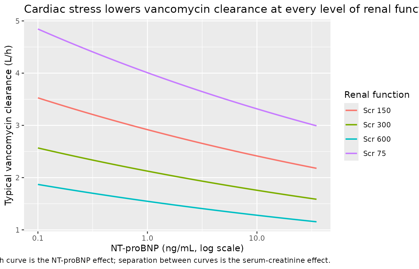
The paper’s contribution is the NT-proBNP term. Over the range simulated in Table S2 it changes clearance by a factor of 1.46, which is modest per unit but material because NT-proBNP spans more than two orders of magnitude in this cohort.

tibble(NTPROBNP = 10^seq(log10(0.1), log10(35), length.out = 60)) |>
  mutate(
    `Scr 75`  = 3.22 * (75  / 80)^-0.458 * (NTPROBNP / 10)^-0.0823,
    `Scr 150` = 3.22 * (150 / 80)^-0.458 * (NTPROBNP / 10)^-0.0823,
    `Scr 300` = 3.22 * (300 / 80)^-0.458 * (NTPROBNP / 10)^-0.0823,
    `Scr 600` = 3.22 * (600 / 80)^-0.458 * (NTPROBNP / 10)^-0.0823
  ) |>
  tidyr::pivot_longer(-NTPROBNP, names_to = "Renal function",
                      values_to = "cl") |>
  ggplot(aes(NTPROBNP, cl, colour = `Renal function`)) +
  geom_line(linewidth = 0.8) +
  scale_x_log10() +
  labs(
    x = "NT-proBNP (ng/mL, log scale)",
    y = "Typical vancomycin clearance (L/h)",
    title = "Cardiac stress lowers vancomycin clearance at every level of renal function",
    caption = paste(
      "Typical 45-year-old, 176 cm, 70 kg male at cystatin C 1.5 mg/L.",
      "Vertical span of each curve is the NT-proBNP effect; separation between",
      "curves is the serum-creatinine effect."
    )
  )

# Deterministic ratios from the printed exponents -- not cohort quantities.
bnp_ratio  <- (0.2 / 10)^-0.0823 / (20 / 10)^-0.0823
scr_ratio  <- (75  / 80)^-0.458  / (600 / 80)^-0.458
sprintf("NT-proBNP 0.2 -> 20 ng/mL changes CL by %.0f%%; Scr 75 -> 600 umol/L by %.1f-fold",
        100 * (bnp_ratio - 1), scr_ratio)
#> [1] "NT-proBNP 0.2 -> 20 ng/mL changes CL by 46%; Scr 75 -> 600 umol/L by 2.6-fold"

stopifnot(bnp_ratio > 1, scr_ratio > 2)

Assumptions and deviations

Errata and internal inconsistencies in the source

• The Conclusion says “sigmoid”, the final model is a power model. The Conclusion states that serum creatinine “was confirmed to be a significant covariate for CL via a sigmoid model”. The final model does not use a sigmoid. The Online Resource Results section explains what happened: both a power model (Equation S3) and a sigmoid model (Equation S4) were fitted for serum creatinine, and although the sigmoid gave the larger OFV drop (462.93 vs 426.83), it inflated the typical clearance from 3.98 to 8.69 L/h and was not retained. Table 2’s Model 2 records the power model’s 426.83, Table 3 reports FScr_CL as a single exponent, and the deposited control stream codes FScr_CL=(Scr/80)**FScr_CL1. The power model is used here; the Conclusion sentence is an error.
• “The standard fat mass (FAT_STD) … was 56.1 kg.” The Online Resource labels 56.1 kg as the standard fat mass of a 70 kg, 176 cm male. It is the standard fat-free mass: Equation S6 evaluated at those values returns 56.13, and the control stream divides by 56.1 immediately after computing FFM. The fat mass of that subject is 70 - 56.1 = 13.9 kg. The model uses 56.1 as the fat-free-mass standard, as the code does.
• NT-proBNP is reported in ng/mL, not the usual pg/mL. A cohort median of 1.095 ng/mL is 1095 pg/mL. The centring constant of 10 ng/mL is therefore 10,000 pg/mL. Anyone supplying data in the conventional clinical unit must divide by 1000 first.

Choices made because the source is silent

• Number of occasions for the IOV terms. Ding 2026 reports both IOV magnitudes (Table 3) and confirms exactly two IOV variances through the 2-df OFV drop for Model 8 (Table 2), but never states how many occasions were defined or how an occasion was delimited; the deposited stream is a prediction stream that drops IOV entirely and carries no occasion column. Four occasions are encoded, covering the cohort’s median of three samples per patient, with occasions 2-4 fixed to the first occasion’s variance in the manner of NONMEM’s $OMEGA BLOCK(1) SAME. A user with more sampling occasions can extend the pattern. Records with OCC outside 1-4 – including OCC = 0, used in the dosage-strategy section above – receive no interoccasion variability.
• Cystatin C and neutrophil count for the virtual standard patient. The paper specifies only age, height, weight and sex for the patient used in the dosage-strategy simulation, plus the serum-creatinine and NT-proBNP levels that define each scenario. Cystatin C and neutrophil count are set to the model’s centring values (1.5 mg/L and 8.0 x 10^9/L) so their covariate factors are exactly 1. This is corroborated rather than assumed: it reproduces all 144 Table S2 cells to a median of well under one percentage point and reselects all twelve Table 4 regimens, neither of which would survive a different cystatin C value.
• No interoccasion variability in the dosage-strategy replication. The deposited prediction control stream omits IOV, and the reproduction is measurably closer to Table S2 without it, so the replication above uses clearance IIV only.
• Virtual cohort covariate distributions. Table 1 reports medians and 2.5-97.5 percentiles but no distributional family and no correlations between covariates. Age and height are drawn normal; weight and the four laboratory values are drawn lognormal, anchored on the reported median with a log-scale SD implied by the percentile range. Covariates are drawn independently, which is certainly wrong in detail – serum creatinine and cystatin C are strongly correlated in reality, and Figs. S1-S8 of the Online Resource are scatter plots of exactly those correlations – but the cohort is used only for the profile figure and the NCA identity check, neither of which depends on the joint structure.
• Assay indicator. Simulations use ASSAY_CMIA = 1, the method that supplied 94.8% of the observed concentrations.

Not reproduced

• Ding 2026 reports no non-compartmental parameters, so there is no published NCA table to compare against. The NCA section validates the simulation against the closed-form dose / CL and log(2) * V / CL identities instead.
• The goodness-of-fit plots (Figure 1) and the visual predictive check (Figure 2) are diagnostics of the fit to the original observed data, which are not public (“available from the corresponding author on reasonable request”). The simulated profile above is comparable in shape and spread to Figure 2b but is not a like-for-like VPC.