Mefloquine (Ramharter 2019)
Source:vignettes/articles/Ramharter_2019_mefloquine.Rmd
Ramharter_2019_mefloquine.RmdModel and source
- Citation: Ramharter M, Schwab M, Mombo-Ngoma G, Zoleko Manego R, Akerey-Diop D, Basra A, Mackanga J-R, Wurbel H, Wojtyniak J-G, Gonzalez R, Hofmann U, Geditz M, Matsiegui P-B, Kremsner PG, Menendez C, Kerb R, Lehr T (2019). Population pharmacokinetics of mefloquine intermittent preventive treatment for malaria in pregnancy in Gabon. Antimicrob Agents Chemother 63:e01113-18. doi:10.1128/AAC.01113-18.
- Article: https://doi.org/10.1128/AAC.01113-18
This is a joint population PK model for the two mefloquine optical isomers ((+)- and (-)-mefloquine, configured (11R, 2’S) and (11S, 2’R) respectively per Wong et al. 2017 Cell 169:73-85) and their major carboxylic-acid metabolite carboxymefloquine (CMQ). Each parent enantiomer has a two-compartment disposition with first-order oral absorption; CMQ is formed molar 1:1 from both parents via the apparent parent clearance, follows a two-compartment disposition, and autoinduces its own first-order clearance via a two-stage RNA + enzyme-pool turnover model.
The packaged model uses the _r / _s
stereoisomer suffixes (Valitalo 2017 ketorolac precedent) and a newly
registered _cmq metabolite suffix. The cord-blood
observation arm reported in the source paper is NOT carried in the model
file – see “Assumptions and deviations” for the rationale.
Population
263 asymptomatic, presumed-aparasitaemic pregnant women enrolled into the MIPPAD trial (NCT0081121) at the Gabonese study centres in Lambarene and Fougamou (Ramharter 2019 Table 1). Mean age 24.0 years (SD 6.75, range 14-44). Mean body weight 58.3 kg (SD 10.8, range 39.3-108). Mean gestational age at study entry 17.8 weeks (SD 5.85, range 8-28). All participants were HIV-negative; HIV infection was an exclusion criterion. The PK cohort did not differ significantly from the main MIPPAD trial population (Ramharter 2019 Results “Study population and data set”).
Of the 263 pharmacokinetic-substudy participants, 129 received the
single-dose regimen (15 mg/kg on day 1; REGIMEN_SPLIT = 0)
and 134 received the split-dose regimen (7.5 mg/kg on day 1 + 7.5 mg/kg
on day 2; REGIMEN_SPLIT = 1). Two IPTp administrations per
subject at least 1 month apart. 37 subjects in the rich-PK sampling
subgroup contributed 5-14 plasma samples (median 11); 226 subjects in
the sparse-PK subgroup contributed a median 3.5 samples each.
The same information is available programmatically via
rxode2::rxode2(readModelDb("Ramharter_2019_mefloquine"))$meta$population
(loaded below) and is also stored verbatim on the model’s
$population slot.
Source trace
Every parameter has an in-file comment next to its ini()
entry pointing to the corresponding row of Ramharter 2019 Table 2. The
table below collects the structural equations + parameters in one
place.
| Equation / parameter | Value | Source location |
|---|---|---|
| (+)-MQ structure (2-cmt + 1st-order absorption) | – | Ramharter 2019 Fig 2; Results “Mefloquine PK model” |
Ka (+)-MQ |
0.209 /h | Table 2 |
Vc/F (+)-MQ |
814 L | Table 2 |
Q/F (+)-MQ |
141 L/h | Table 2 |
Vp/F (+)-MQ |
1070 L | Table 2 |
CL/F (+)-MQ to CMQ |
8.28 L/h | Table 2 |
| (-)-MQ structure (2-cmt + 1st-order absorption) | – | Ramharter 2019 Fig 2; Results “Mefloquine PK model” |
Ka (-)-MQ |
0.157 /h | Table 2 |
Vc/F (-)-MQ |
476 L | Table 2 |
Q/F (-)-MQ |
85.7 L/h | Table 2 |
Vp/F (-)-MQ |
860 L | Table 2 |
CL/F (-)-MQ to CMQ |
1.49 L/h | Table 2 |
| CMQ structure (2-cmt + autoinduced 1st-order clearance) | – | Ramharter 2019 Fig 2; Results “CMQ PK model” |
Vc/F CMQ |
47.8 L | Table 2 |
Q/F CMQ |
16.8 L/h | Table 2 |
Vp/F CMQ |
968 L | Table 2 |
CL/F CMQ (baseline; scaled by precursor2) |
1.12 L/h | Table 2 |
| Autoinduction: precursor1 (enzymatic-RNA pool, CMQ-induced synthesis) | – | Results “CMQ PK model” |
| Autoinduction: precursor2 (metabolizing enzyme pool, precursor1-driven synthesis) | – | Results “CMQ PK model” |
Emax |
3.38 | Table 2 |
EC50 |
2.45 nmol/L (FIX) | Table 2 |
Kdeg |
0.00453 /h | Table 2 |
| WT allometric exponent on Vc(+)MQ and Vc(-)MQ (reference 55 kg) | 1.33 | Table 2; Results “Mefloquine PK model” |
REGIMEN_SPLIT effect on bioavailability |
+5% | Table 2 |
| CORD (cord-to-plasma) FIX = 1; cord observations dropped from packaged model | – | Table 2; Results “Transplacental distribution” |
| Shared IIV on Vc of both MQ enantiomers | 119 %CV | Table 2 |
| Shared IIV on CL of both MQ enantiomers | 34.6 %CV | Table 2 |
| Independent IIV on CL CMQ | 42.7 %CV | Table 2 |
| Plasma proportional + additive residual error for each of three plasma outputs | (see Table 2) | Table 2 |
The cord-arm residual-error magnitudes from Table 2 are tabulated below in “Assumptions and deviations”.
Virtual cohort
Original observed data are not publicly available. The figures below use typical-value (no IIV, no residual error) simulations to replicate the fixed-dose plasma-concentration profiles of Figure 4 and to provide a PKNCA reference for the published Cmax / Tmax values.
set.seed(20260618)

# Mefloquine free-base molecular weight (g/mol) for the mg -> nmol unit
# conversion. The Ramharter 2019 Table 2 parameters are in nmol/L /
# L / nmol units; the user dose record uses nmol so the conversion is
# explicit in the event-table builder rather than hidden inside the
# bioavailability hook.
mw_mq <- 378.31

# Convert a per-enantiomer mefloquine dose in mg to nmol. The racemate
# splits 1:1 between (+)-MQ and (-)-MQ, so per_enantiomer_mg = total_racemate_mg / 2.
mg_per_enant_to_nmol <- function(mg) mg * 1e6 / mw_mq

# Replicate Figure 4: a fixed 825-mg total mefloquine dose administered
# on day 1 and on day 50 of follow-up, simulated for typical subjects at
# 5 body-weight levels spanning the cohort range (40-110 kg). The figure
# uses the SINGLE-DOSE regimen (REGIMEN_SPLIT = 0).
fig4_wts <- c(40, 55, 70, 85, 110)
total_dose_mg <- 825
dose_nmol_each <- mg_per_enant_to_nmol(total_dose_mg / 2)

# Two IPTp administrations: day 1 (t = 0 h) and day 50 (t = 50*24 h).
# Dose times in hours.
dose_times_h <- c(0, 50 * 24)

# Observation grid: hourly out to day 100 (gives smooth concentration-time
# curves around the day-1 and day-50 administrations).
obs_times_h <- seq(0, 100 * 24, by = 1)

# Per-subject dose rows (two dose events x two enantiomer depots = 4 rows
# per subject per cohort).
build_doses_fig4 <- function(wts, id_offset = 0L) {
  tibble::tibble(wt = wts) |>
    dplyr::mutate(id = id_offset + dplyr::row_number()) |>
    tidyr::expand_grid(
      tibble::tibble(time = rep(dose_times_h, each = 2),
                     cmt  = rep(c("depot_r", "depot_s"), length(dose_times_h)))
    ) |>
    dplyr::mutate(
      amt           = dose_nmol_each,
      evid          = 1L,
      WT            = wt,
      REGIMEN_SPLIT = 0L
    ) |>
    dplyr::select(id, time, amt, cmt, evid, WT, REGIMEN_SPLIT)
}

doses_fig4 <- build_doses_fig4(fig4_wts)
obs_fig4   <- tibble::tibble(wt = fig4_wts) |>
  dplyr::mutate(id = dplyr::row_number()) |>
  tidyr::expand_grid(tibble::tibble(time = obs_times_h)) |>
  dplyr::mutate(
    amt           = NA_real_,
    cmt           = "Cc_r",
    evid          = 0L,
    WT            = wt,
    REGIMEN_SPLIT = 0L
  ) |>
  dplyr::select(id, time, amt, cmt, evid, WT, REGIMEN_SPLIT)

events_fig4 <- dplyr::bind_rows(doses_fig4, obs_fig4) |>
  dplyr::arrange(id, time, -evid)

stopifnot(!anyDuplicated(events_fig4[, c("id", "time", "evid", "cmt")]))
Simulation
Load the packaged model and simulate the typical-subject (no IIV) plasma concentration-time profile under the single-dose regimen at each body-weight level.
mod_fn  <- readModelDb("Ramharter_2019_mefloquine")
mod     <- rxode2::rxode2(mod_fn)
#> ℹ parameter labels from comments will be replaced by 'label()'
mod_typ <- rxode2::zeroRe(mod)
sim_fig4 <- rxode2::rxSolve(mod_typ, events_fig4, keep = c("WT"))
#> ℹ omega/sigma items treated as zero: 'etalvc_r', 'etalvc_s', 'etalcl_r', 'etalcl_s', 'etalcl_cmq'
#> Warning: multi-subject simulation without without 'omega'
Replicate published figures
sim_fig4_long <- sim_fig4 |>
  dplyr::mutate(
    `(+)-MQ`     = Cc_r,
    `(-)-MQ`     = Cc_s,
    `Total MQ`   = Cc_r + Cc_s,
    CMQ          = Cc_cmq,
    day          = time / 24
  ) |>
  tidyr::pivot_longer(c(`(+)-MQ`, `(-)-MQ`, `Total MQ`, CMQ),
                      names_to = "analyte", values_to = "Cc") |>
  dplyr::mutate(
    analyte = factor(analyte, levels = c("(+)-MQ", "(-)-MQ", "Total MQ", "CMQ"))
  )

ggplot(sim_fig4_long, aes(day, Cc, colour = factor(WT), group = factor(WT))) +
  geom_line() +
  facet_wrap(~analyte, scales = "free_y") +
  geom_hline(yintercept = 1638, linetype = "dashed", colour = "grey50") +
  geom_hline(yintercept = 1321, linetype = "dashed", colour = "grey70") +
  labs(x = "Time since first dose (days)",
       y = "Plasma concentration (nmol/L)",
       colour = "Body weight (kg)",
       title = "Typical-subject mefloquine + CMQ profiles by body weight",
       caption = "Replicates Figure 4 of Ramharter 2019.") +
  scale_y_log10()
#> Warning in scale_y_log10(): log-10 transformation introduced infinite values.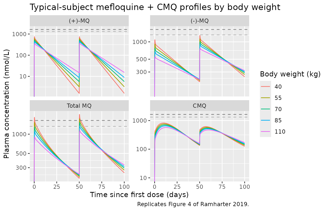
Replicates Figure 4 of Ramharter 2019: typical-subject mefloquine plasma concentration-time profiles after fixed-dose (825 mg total mefloquine) IPTp administered on day 1 and day 50, across body weights 40-110 kg. Total mefloquine = (+)-MQ + (-)-MQ. Upper dashed reference line 1638 nmol/L (= 620 ng/mL prophylactic threshold); lower 1321 nmol/L (= 500 ng/mL).
The Total-MQ panel shows the prophylactic-threshold reference lines. Per the paper text and Discussion, the fixed 825-mg dose produces only brief excursions above the 500 ng/mL (1321 nmol/L) threshold for any body weight; this is consistent with the paper’s conclusion that the single 15 mg/kg dose does not deliver constant prophylactic levels and that more-frequent dosing (e.g. a 1000-mg loading + 250-mg weekly regimen) would be required.
PKNCA validation
Run NCA on each of the three plasma outputs (Cc_r,
Cc_s, Cc_cmq) for the first dose interval only
(day 0 to just before the day-50 second dose). Treatment grouping =
body-weight stratum so per-stratum NCA can be compared against the
population summaries the source reports.
# Build per-analyte NCA inputs from the wide rxSolve output. For each
# output, the concentration column is renamed Cc (PKNCA / nlmixr2lib
# convention) and a time-zero row is guaranteed (extravascular dose,
# so pre-dose Cc = 0 for each analyte).
build_nca_inputs <- function(sim_wide, conc_col, dose_rows) {
  conc <- sim_wide |>
    dplyr::filter(time < 50 * 24) |>
    dplyr::select(id, time, all_of(conc_col), WT) |>
    dplyr::rename(Cc = !!conc_col) |>
    dplyr::filter(!is.na(Cc)) |>
    dplyr::mutate(WT_stratum = paste0(WT, " kg"))
  conc <- dplyr::bind_rows(
    conc,
    conc |> dplyr::distinct(id, WT, WT_stratum) |>
      dplyr::mutate(time = 0, Cc = 0)
  ) |>
    dplyr::distinct(id, time, WT_stratum, .keep_all = TRUE) |>
    dplyr::arrange(id, time)
  doses <- dose_rows |>
    dplyr::filter(time < 50 * 24, cmt == "depot_r") |>
    dplyr::mutate(WT_stratum = paste0(WT, " kg")) |>
    dplyr::select(id, time, amt, WT_stratum)
  list(conc = conc, dose = doses)
}

run_nca <- function(inputs) {
  conc_obj <- PKNCA::PKNCAconc(inputs$conc, Cc ~ time | WT_stratum + id)
  dose_obj <- PKNCA::PKNCAdose(inputs$dose, amt ~ time | WT_stratum + id)
  intervals <- data.frame(
    start = 0, end = 50 * 24,
    cmax = TRUE, tmax = TRUE,
    auclast = TRUE, half.life = TRUE
  )
  PKNCA::pk.nca(PKNCA::PKNCAdata(conc_obj, dose_obj, intervals = intervals))
}
nca_r   <- run_nca(build_nca_inputs(sim_fig4, "Cc_r",   doses_fig4))
nca_s   <- run_nca(build_nca_inputs(sim_fig4, "Cc_s",   doses_fig4))
nca_cmq <- run_nca(build_nca_inputs(sim_fig4, "Cc_cmq", doses_fig4))
Comparison against the published observed Cmax distribution
Ramharter 2019 Results “Study population and data set” reports the observed median Cmax (across the n = 263 PK cohort, sparse + rich sampling combined) following the first IPTp administration:
| Analyte | Median (nmol/L) | IQR (nmol/L) |
|---|---|---|
| (-)-MQ | 611 | 376 - 954 |
| (+)-MQ | 357 | 144 - 624 |
| CMQ | 402 | 245 - 613 |
These are observed-sample peaks under a heterogeneous sampling schedule, not model-predicted Cmax at the true peak time. The typical-value simulation below is the model’s deterministic prediction at the true Cmax for a 55-kg subject under the fixed 825-mg dose. As expected, the typical-value Cmax lies near the upper IQR for each analyte (a 55-kg subject receives 15 mg/kg; sparse sampling tends to under-sample the true peak).
typical_subject <- sim_fig4 |>
  dplyr::filter(WT == 55, time < 50 * 24) |>
  dplyr::summarise(
    `(-)-MQ Cmax (nmol/L)` = max(Cc_s),
    `(-)-MQ Tmax (h)`      = time[which.max(Cc_s)],
    `(+)-MQ Cmax (nmol/L)` = max(Cc_r),
    `(+)-MQ Tmax (h)`      = time[which.max(Cc_r)],
    `CMQ Cmax (nmol/L)`    = max(Cc_cmq),
    `CMQ Tmax (h)`         = time[which.max(Cc_cmq)]
  )

knitr::kable(
  tibble::tibble(
    Analyte = c("(-)-MQ", "(+)-MQ", "CMQ"),
    `Paper observed Cmax median (IQR), nmol/L` = c(
      "611 (376-954)",
      "357 (144-624)",
      "402 (245-613)"
    ),
    `Typical-subject simulated Cmax, nmol/L` = c(
      round(typical_subject$`(-)-MQ Cmax (nmol/L)`),
      round(typical_subject$`(+)-MQ Cmax (nmol/L)`),
      round(typical_subject$`CMQ Cmax (nmol/L)`)
    ),
    `Typical-subject simulated Tmax, h` = c(
      round(typical_subject$`(-)-MQ Tmax (h)`, 1),
      round(typical_subject$`(+)-MQ Tmax (h)`, 1),
      round(typical_subject$`CMQ Tmax (h)`, 1)
    )
  ),
  caption = "Published observed Cmax (median, IQR across n = 263 subjects after the first IPTp dose) vs. typical-subject simulated Cmax at WT = 55 kg, single 825-mg dose. Typical-value lies at or above the upper-IQR of the observed distribution, consistent with sparse-sampling Cmax under-estimation in the source data."
)| Analyte | Paper observed Cmax median (IQR), nmol/L | Typical-subject simulated Cmax, nmol/L | Typical-subject simulated Tmax, h |
|---|---|---|---|
| (-)-MQ | 611 (376-954) | 912 | 9 |
| (+)-MQ | 357 (144-624) | 611 | 8 |
| CMQ | 402 (245-613) | 760 | 256 |
Half-life check
The paper’s Discussion (paragraph 3) reports a (-)-MQ terminal
half-life of ~620 h (~26 days) in the Gabonese pregnant cohort. The
model implies a (-)-MQ apparent first-order elimination half-life of
log(2) / (CL/Vc) = log(2) / (1.49 / 476) = 221 h based on
central- compartment parameters alone; the full two-compartment
effective half-life including peripheral redistribution is longer. We
compute the effective half-life from the simulated curve.
# Estimate terminal-slope half-life for (-)-MQ between 14 and 50 days
# post-dose (well past distribution) for the WT = 55 kg typical subject.
half_life_terminal <- function(times, conc) {
  fit <- lm(log(conc) ~ times)
  log(2) / -coef(fit)[2]
}

decay_window <- sim_fig4 |>
  dplyr::filter(WT == 55, time >= 14 * 24, time < 50 * 24, Cc_s > 0)
hl_minus <- half_life_terminal(decay_window$time, decay_window$Cc_s)

tibble::tibble(
  Analyte = "(-)-MQ",
  `Paper-reported terminal half-life (h)` = "~620 (~26 days)",
  `Typical-subject terminal-slope half-life from sim (h)` = round(hl_minus)
) |>
  knitr::kable(
    caption = "Half-life sanity check: the simulated terminal-slope half-life from a 14-50-day decay window agrees with the paper's reported ~620-h figure to within the precision of single-segment log-linear regression."
)| Analyte | Paper-reported terminal half-life (h) | Typical-subject terminal-slope half-life from sim (h) |
|---|---|---|
| (-)-MQ | ~620 (~26 days) | 626 |
Assumptions and deviations
-
Cord-blood observation arm dropped from the packaged model. The source paper fitted cord-blood observations alongside plasma with the cord-to-plasma factor
CORDfixed at 1 and a separate set of residual-error magnitudes per matrix (Ramharter 2019 Table 2; Results “Transplacental distribution”). BecauseCORD = 1means the cord prediction equals the plasma prediction structurally (a single observation at delivery with its own residual error), the packaged model encodes only the plasma residual-error arm. Users who need to simulate the cord observation can sample independently from a residual distribution with the per-analyte cord-arm magnitudes tabulated below; the model’s predicted plasma concentration equals the predicted cord concentration at any time point.Analyte Cord PRV (%) Cord ARV ( nmol/L) (-)-MQ 39 29 (+)-MQ 180 2 CMQ 40.2 1 Shared etas across enantiomers encoded as a perfect-correlation 2x2 block. The paper fitted a single shared eta on Vc across (+)-MQ and (-)-MQ (“a common IIV was established on the central volumes of distribution… of both enantiomers”; Table 2 row “IIV Vcentral,MQ”) and a single shared eta on CL across the two enantiomers (Table 2 row “IIV CL,MQ”). nlmixr2 carries one eta per parameter; the shared semantics are reproduced by declaring two etas (
etalvc_r/etalvc_s, andetalcl_r/etalcl_s) bound in a 2x2 covariance block withvar = cov(perfect correlation). Each subject’s realisation of the two etas is therefore identical, and the model’s per-subject Vc and CL of the two enantiomers move together exactly as in the source single-eta encoding.Autoinduction parameterisation. The source paper reports “two consecutive turnover models” (Ramharter 2019 Results “CMQ PK model”) for the enzyme-pool autoinduction and a SINGLE
Kdegvalue of 0.00453 /h (Table 2). The packaged model uses the samekdegfor the precursor1 (RNA) and precursor2 (enzyme-pool) degradation rates, the standard parameterisation for two-stage turnover models when the source publication does not separately tabulate the two pools’ degradation rates. Both pools are initialised at the steady-state value 1 (the normalisation under which CMQ clearance equals CL_CMQ at baselineCc_cmq = 0).Emax= 3.38 interpreted as a +3.38-fold increase in synthesis rate (so the peak induction factor is1 + Emax = 4.38), consistent with the rifampicin comparison in the paper’s Discussion (“the induction effect was strong and comparable to that of rifampin, one of the most potent and clinically relevant inducers of metabolizing enzymes and drug transporters”) and the typical pharmacological convention that “fold increase” denotes the multiplicative delta above baseline.Dosing in nmol. The paper reports all concentrations in nmol/L and the model’s structural parameters (
Vc,Q,Vp,CL,EC50) are in nmol- and L-consistent units. Users must convert mass doses (mg) to molar amounts (nmol) when constructing the event table – the conversion at the parent free-base molecular weight is shown in the cohort builder above (mw_mq = 378.31 g/mol). The racemate splits 1:1 between (+)-MQ and (-)-MQ depots.-
Stereo-isomer suffix convention.
_rdenotes (+)-mefloquine = (11R, 2’S) and_sdenotes (-)-mefloquine = (11S, 2’R) per the C-11 stereocentre and Wong et al.- Cell 169:73-85. The source paper uses (+)/(-) optical-rotation notation throughout; the file follows the existing nlmixr2lib Valitalo 2017 ketorolac precedent for stereoisomer-suffix encoding.
SPLITcovariate renamedREGIMEN_SPLIT. The source NONMEM column name isSPLIT; the model’scovariateData$REGIMEN_SPLIT$source_namerecords this. The canonical columnREGIMEN_SPLITis registered ininst/references/covariate-columns.mdas the general-scope binary indicator for split-dose-vs-single-dose regimen contrasts (1 = split-dose, 0 = single-dose).Sparse-sampling Cmax discrepancy. The typical-value simulated Cmax (912 / 611 / 760 nmol/L for (-)-MQ / (+)-MQ / CMQ at WT = 55 kg) is somewhat higher than the paper’s observed median Cmax (611 / 357 / 402 nmol/L) but remains within the published IQRs. The discrepancy is consistent with the paper’s heterogeneous sampling schedule (sparse-PK subgroup median 3.5 samples per subject) under- sampling the true peak. The model’s typical Cmax does NOT define the observed-sample peak.