Ciclosporin (Wilhelm 2012)
Source:vignettes/articles/Wilhelm_2012_ciclosporin.Rmd
Wilhelm_2012_ciclosporin.RmdModel and source
- Citation: Wilhelm AJ, de Graaf P, Veldkamp AI, Janssen JJWM, Huijgens PC, Swart EL. Population pharmacokinetics of ciclosporin in haematopoietic allogeneic stem cell transplantation with emphasis on limited sampling strategy. Br J Clin Pharmacol. 2012;73(4):553-563. doi:10.1111/j.1365-2125.2011.04116.x.
- Description: Two-compartment population PK model for ciclosporin (CsA) in adults undergoing haematopoietic allogeneic stem cell transplantation, with first-order oral absorption + lag time and a 3 h intravenous infusion directly into the central compartment (Wilhelm 2012). Twenty subjects on routine fluconazole antimycotic prophylaxis (a CYP3A4 inhibitor) were included; ciclosporin was assayed in whole blood by FPIA (AxSYM, Abbott). Body weight, body surface area, co-medication with CYP3A4 inducers and co-medication with CYP3A4 inhibitors were tested but none reached statistical or clinical significance, so no covariates are retained in the final model. Inter-individual variability was reported on every PK parameter (CL, Vc, Q, Vp, ka, F, tlag); the paper estimated a full omega variance-covariance matrix but did not publish the off-diagonal elements, so the packaged model uses diagonal IIVs only (see vignette Assumptions and deviations).
- Article: https://doi.org/10.1111/j.1365-2125.2011.04116.x
Population
Wilhelm 2012 enrolled 20 adults undergoing allogeneic haematopoietic stem cell transplantation (HSCT) at VU University Medical Center, Amsterdam, between January 2005 and February 2008. Demographics (Table 1): median age 54 years (range 37-66), median body weight 84 kg (range 53-110), median body surface area 2.02 m^2 (1.48-2.43), 13 male / 7 female. The underlying haematological malignancies were acute myeloid leukaemia (n=7), non-Hodgkin lymphoma (n=6), chronic lymphoblastic leukaemia (n=2) and other diagnoses (n=5). Conditioning regimens were fludarabine + cyclophosphamide (n=10), fludarabine + total-body irradiation (n=6), or cyclophosphamide + total-body irradiation (n=4). All subjects received fluconazole 50 mg once daily as routine antimycotic prophylaxis throughout the sampling period; fluconazole is a moderate CYP3A4 inhibitor that the authors highlight as the most likely driver of the relatively low clearance reported here compared with non-HSCT renal/liver transplant cohorts (Discussion, page referencing Schultz et al. and Dotti et al.).
Ciclosporin was administered as a 2.5 mg/kg intravenous infusion over 3 h at the start of the conditioning scheme. After tolerance to oral intake was established, dosing was switched to twice-daily oral Neoral microemulsion at clinician-adjusted doses (mean 2.77 +/- 0.81 mg/kg per dose during the recorded oral profile) targeting trough concentrations of 200-400 ug/L. Whole-blood ciclosporin was assayed by fluorescence polarization immunoassay (FPIA, AxSYM Abbott) with LLOQ 80 ug/L and intra-assay CV below 10%; 436 concentration measurements were available for the popPK analysis.
The same information is available programmatically via
rxode2::rxode(readModelDb("Wilhelm_2012_ciclosporin"))$population.
Source trace
The per-parameter origin is recorded as a trailing in-file comment
next to each ini() entry in
inst/modeldb/specificDrugs/Wilhelm_2012_ciclosporin.R. The
table below collects them in one place for review.
| Equation / parameter | Value | Source location (Wilhelm 2012) |
|---|---|---|
| Two-compartment open model with first-order oral absorption + lag time | n/a | Methods ‘Basic pharmacokinetic model’; Results Table 2 |
| IV dosing: 3 h infusion into central compartment | n/a | Methods ‘Basic pharmacokinetic model’ (‘I.v. administration was modelled as a 3 h infusion in the central compartment’) |
| Combined additive + proportional residual error | n/a | Methods ‘Basic pharmacokinetic model’ |
lcl (CL) |
log(21.9) L/h | Table 3, RSD 5.2% |
lvc (V1) |
log(16.6) L | Table 3, RSD 8.7% (abstract reports 18.3 L matching the bootstrap median ~18; the formal final estimate from Table 3 is 16.6 L) |
lq (Q) |
log(24.2) L/h | Table 3, RSD 9.3% |
lvp (V2) |
log(59.0) L | Table 3, RSD 8.8% |
lka (ka) |
log(0.280) 1/h | Table 3, RSD 14.6% |
lfdepot (F) |
log(0.710) | Table 3, RSD 9.9% |
ltlag (tlag) |
log(0.440) h | Table 3, RSD 5.5% |
etalcl variance |
log(1 + 0.222^2) = 0.04812 | Table 3 IIV CL 22.2% CV (RSD 55%) |
etalvc variance |
log(1 + 0.269^2) = 0.06988 | Table 3 IIV V1 26.9% CV (RSD 53%) |
etalq variance |
log(1 + 0.282^2) = 0.07650 | Table 3 IIV Q 28.2% CV (RSD 73%) |
etalvp variance |
log(1 + 0.306^2) = 0.08947 | Table 3 IIV V2 30.6% CV (RSD 62%) |
etalka variance |
log(1 + 0.438^2) = 0.17559 | Table 3 IIV ka 43.8% CV (RSD 66%) |
etalfdepot variance |
log(1 + 0.250^2) = 0.06062 | Table 3 IIV F 25.0% CV (RSD 64%) |
etaltlag variance |
log(1 + 0.181^2) = 0.03224 | Table 3 IIV tlag 18.1% CV (RSD 90%) |
addSd (ug/L) |
65 | Table 3 ‘Additive error (ug/L)’ = 65 (RSD 86%) |
propSd (fraction) |
0.088 | Table 3 ‘Proportional error (%)’ = 8.8 (RSD 84%) |
Virtual cohort
The original individual-level data are not publicly available. The virtual cohort below mirrors the published demographics (n=20 HSCT recipients, weight 53-110 kg) at a larger sample size (n=200) so that simulated geometric-mean NCA parameters can be compared with the cohort means reported in the paper without small-sample noise.
Build event tables
Two cohorts are simulated:
- IV – a single 2.5 mg/kg infusion over 3 h into the central compartment, with observations over 12 h post-start, mirroring the IV profile collected on day 1 of conditioning.
- Oral (steady state) – 2.77 mg/kg twice daily (Neoral) for 10 days to reach steady state, then a densely-sampled 12 h observation window on the morning of day 11 (the last dosing interval), mirroring the oral profile collected after tolerance to oral intake was established.
IDs are offset between the two cohorts so subsequent
bind_rows() keeps them disjoint per the vignette-template
guidance.
make_iv_cohort <- function(cohort, dose_mg_per_kg = 2.5,
                           infusion_h = 3, obs_grid = NULL,
                           id_offset = 0L) {
  if (is.null(obs_grid)) obs_grid <- sort(unique(c(seq(0, 12, by = 0.25),
                                                   c(0.25, 0.5, 1, 1.5,
                                                     2.5, 4, 4.5, 6.5,
                                                     9, 10, 12))))
  cohort |>
    dplyr::mutate(id = id + id_offset,
                  amt = dose_mg_per_kg * WT) |>
    dplyr::group_by(id) |>
    dplyr::group_modify(function(df, key) {
      dplyr::bind_rows(
        # IV 3 h infusion to central: amt = dose, rate = dose/3
        tibble::tibble(time  = 0,
                       amt   = df$amt,
                       rate  = df$amt / infusion_h,
                       evid  = 1L,
                       cmt   = "central",
                       WT    = df$WT,
                       cohort = "IV 2.5 mg/kg over 3 h"),
        tibble::tibble(time  = obs_grid,
                       amt   = 0,
                       rate  = 0,
                       evid  = 0L,
                       cmt   = "Cc",
                       WT    = df$WT,
                       cohort = "IV 2.5 mg/kg over 3 h")
      )
    }) |>
    dplyr::ungroup() |>
    dplyr::arrange(id, time, dplyr::desc(evid))
}

make_oral_ss_cohort <- function(cohort, dose_mg_per_kg = 2.77,
                                tau = 12, n_days = 10,
                                obs_grid = NULL, id_offset = 0L) {
  if (is.null(obs_grid)) obs_grid <- sort(unique(c(seq(0, 12, by = 0.1),
                                                   c(0.25, 0.5, 0.75, 1,
                                                     1.5, 2, 2.5, 3,
                                                     5, 8, 12))))
  ss_offset <- tau * (2 * n_days - 1)   # time of the last (morning) dose
  cohort |>
    dplyr::mutate(id = id + id_offset,
                  amt = dose_mg_per_kg * WT) |>
    dplyr::group_by(id) |>
    dplyr::group_modify(function(df, key) {
      dose_times <- seq(0, by = tau, length.out = 2 * n_days)
      dplyr::bind_rows(
        tibble::tibble(time  = dose_times,
                       amt   = df$amt,
                       rate  = 0,
                       evid  = 1L,
                       cmt   = "depot",
                       WT    = df$WT,
                       cohort = "Oral 2.77 mg/kg BID (SS)"),
        tibble::tibble(time  = ss_offset + obs_grid,
                       amt   = 0,
                       rate  = 0,
                       evid  = 0L,
                       cmt   = "Cc",
                       WT    = df$WT,
                       cohort = "Oral 2.77 mg/kg BID (SS)")
      )
    }) |>
    dplyr::ungroup() |>
    dplyr::arrange(id, time, dplyr::desc(evid))
}

events_iv   <- make_iv_cohort(cohort,   id_offset =     0L)
events_oral <- make_oral_ss_cohort(cohort, id_offset = 1000L)

events <- dplyr::bind_rows(events_iv, events_oral)
stopifnot(!anyDuplicated(unique(events[, c("id", "time", "evid")])))
Simulation
mod <- readModelDb("Wilhelm_2012_ciclosporin")
sim <- rxode2::rxSolve(mod, events = events, keep = c("cohort", "WT")) |>
  as.data.frame()
#> ℹ parameter labels from comments will be replaced by 'label()'
Replicate Figure 1: 12 h individual concentration-time profiles
Wilhelm 2012 Figure 1 shows the individual whole-blood ciclosporin concentration-time curves for the 20 patients after (A) the 2.5 mg/kg IV dose and (B) oral administration. The simulated profiles below reproduce the same characteristic shapes: a rapid IV peak around the end of infusion, biphasic decline thereafter, and a delayed oral peak near 2 h post-dose.
sim_fig1 <- sim |>
  dplyr::filter(!is.na(Cc)) |>
  dplyr::mutate(tad = ifelse(cohort == "IV 2.5 mg/kg over 3 h",
                             time,
                             time - min(time[cohort == "Oral 2.77 mg/kg BID (SS)"]))) |>
  dplyr::filter(tad >= 0, tad <= 12)

show_ids <- sort(unique(sim_fig1$id))[seq(1, 200, length.out = 20)]

ggplot(sim_fig1 |> dplyr::filter(id %in% show_ids),
       aes(x = tad, y = Cc, group = id)) +
  geom_line(alpha = 0.55, colour = "steelblue") +
  facet_wrap(~ cohort, scales = "free_y") +
  scale_x_continuous(breaks = seq(0, 12, 2)) +
  labs(
    x = "Time after dose (h)",
    y = "Ciclosporin (ug/L)",
    title = "Individual whole-blood ciclosporin concentration-time curves",
    caption = paste0("Replicates Wilhelm 2012 Figure 1 (panel A: IV 2.5 mg/kg over 3 h; ",
                     "panel B: oral 2.77 mg/kg BID at steady state). ",
                     "Twenty subjects shown out of 200 simulated.")
  ) +
  theme_bw()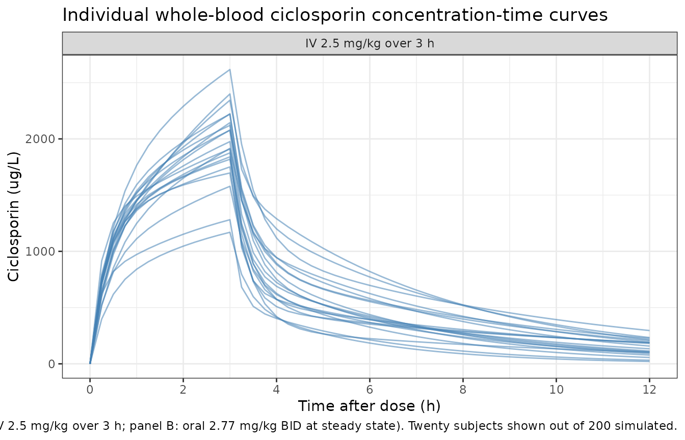
Replicate Figure 2: PRED vs DV / IPRED vs DV diagnostics
Wilhelm 2012 Figure 2 presents log-log scatter plots of (A) population-predicted vs observed and (B) individual-predicted vs observed concentrations. With simulated data the natural analogue is a population VPC: the simulated cohort-level concentration-time envelope should bracket the cohort-typical concentration-time curve.
vpc_iv <- sim |>
  dplyr::filter(cohort == "IV 2.5 mg/kg over 3 h", !is.na(Cc),
                time >= 0, time <= 12) |>
  dplyr::group_by(time) |>
  dplyr::summarise(
    Q05 = quantile(Cc, 0.05, na.rm = TRUE),
    Q50 = quantile(Cc, 0.50, na.rm = TRUE),
    Q95 = quantile(Cc, 0.95, na.rm = TRUE),
    .groups = "drop"
  ) |>
  dplyr::mutate(cohort = "IV 2.5 mg/kg over 3 h", tad = time)

ss_offset_oral <- 12 * (2 * 10 - 1)
vpc_oral <- sim |>
  dplyr::filter(cohort == "Oral 2.77 mg/kg BID (SS)", !is.na(Cc),
                time >= ss_offset_oral, time <= ss_offset_oral + 12) |>
  dplyr::mutate(tad = time - ss_offset_oral) |>
  dplyr::group_by(tad) |>
  dplyr::summarise(
    Q05 = quantile(Cc, 0.05, na.rm = TRUE),
    Q50 = quantile(Cc, 0.50, na.rm = TRUE),
    Q95 = quantile(Cc, 0.95, na.rm = TRUE),
    .groups = "drop"
  ) |>
  dplyr::mutate(cohort = "Oral 2.77 mg/kg BID (SS)")

vpc_combined <- dplyr::bind_rows(vpc_iv, vpc_oral)

ggplot(vpc_combined, aes(x = tad, y = Q50)) +
  geom_ribbon(aes(ymin = Q05, ymax = Q95), alpha = 0.20, fill = "darkorange") +
  geom_line(colour = "darkorange", linewidth = 0.7) +
  facet_wrap(~ cohort, scales = "free_y") +
  scale_x_continuous(breaks = seq(0, 12, 2)) +
  labs(
    x = "Time after dose (h)",
    y = "Ciclosporin (ug/L)",
    title = "Population concentration-time envelopes (median, 5th and 95th percentiles)",
    caption = "Population VPC analogue of Wilhelm 2012 Figure 2 (population-predicted distribution)."
  ) +
  theme_bw()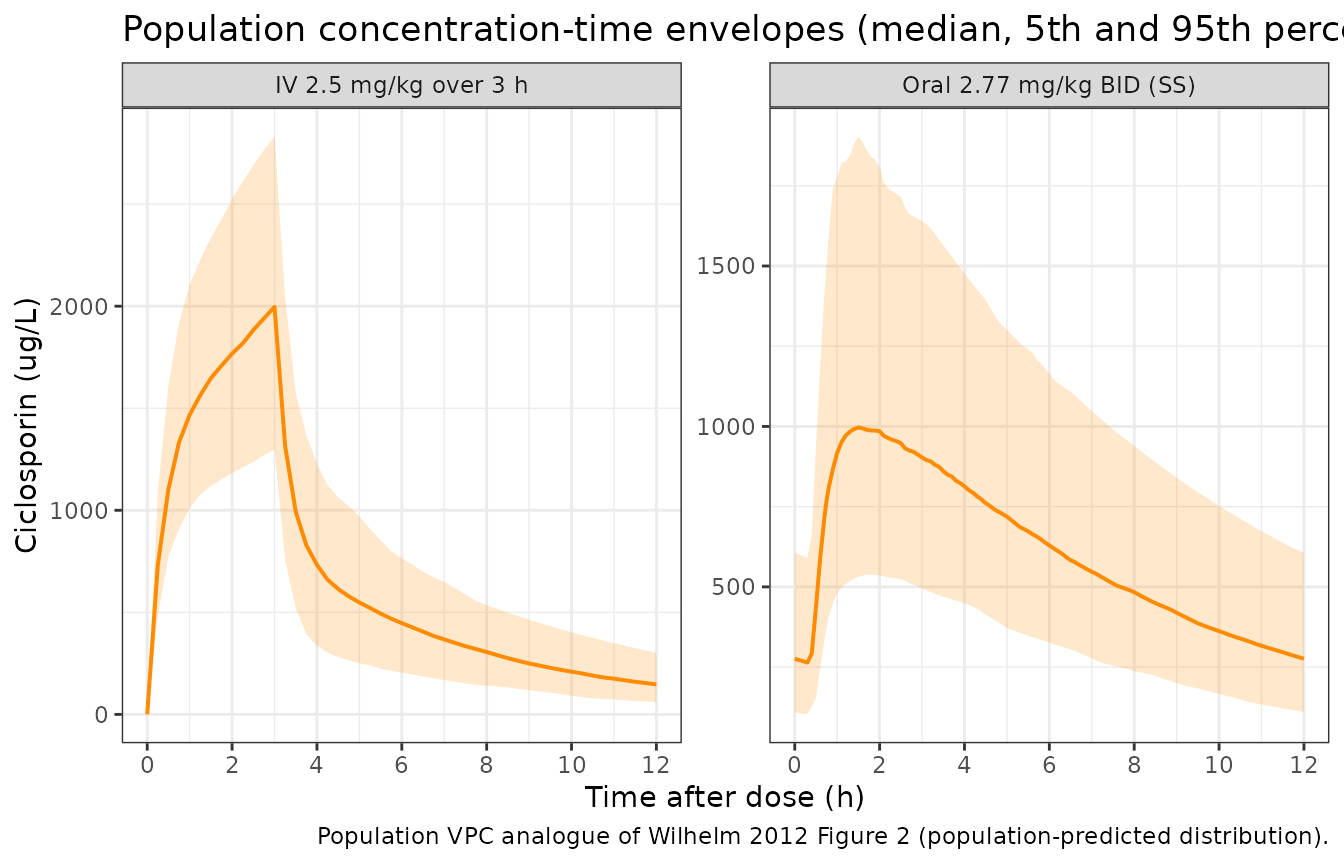
PKNCA validation
The published cohort-mean NCA values listed by Wilhelm 2012 Results (page text following Table 1) are:
- IV 2.5 mg/kg single dose: AUC(0,12 h) = 8580 +/- 2290 ug/L*h, Cmax = 1937 +/- 497 ug/L.
- Oral steady state (mean 2.77 +/- 0.81 mg/kg): AUC(0,12 h) = 7081 +/- 1429 ug/L*h, Cmax = 1080 +/- 284 ug/L, Tmax = 2.0 +/- 0.6 h, C12 = 308 +/- 121 ug/L.
PKNCA is run on the simulated profiles to compute the corresponding NCA endpoints.
sim_iv_nca <- sim |>
  dplyr::filter(cohort == "IV 2.5 mg/kg over 3 h", !is.na(Cc),
                time >= 0, time <= 12) |>
  dplyr::transmute(id, time, Cc,
                   treatment = "IV 2.5 mg/kg over 3 h",
                   amt = NA_real_)

sim_iv_nca <- dplyr::bind_rows(
  sim_iv_nca,
  sim_iv_nca |> dplyr::distinct(id, treatment) |>
    dplyr::mutate(time = 0, Cc = 0)
) |>
  dplyr::distinct(id, treatment, time, .keep_all = TRUE) |>
  dplyr::arrange(id, treatment, time)

dose_iv_nca <- events_iv |>
  dplyr::filter(evid == 1) |>
  dplyr::transmute(id, time, amt, treatment = "IV 2.5 mg/kg over 3 h")

conc_iv <- PKNCA::PKNCAconc(
  data    = sim_iv_nca |> dplyr::select(id, time, Cc, treatment),
  formula = Cc ~ time | treatment + id,
  concu   = "ug/L",
  timeu   = "h"
)
dose_iv <- PKNCA::PKNCAdose(
  data    = dose_iv_nca,
  formula = amt ~ time | treatment + id,
  doseu   = "mg"
)

intervals_iv <- data.frame(
  start    = 0,
  end      = 12,
  cmax     = TRUE,
  tmax     = TRUE,
  auclast  = TRUE
)
nca_iv <- PKNCA::pk.nca(PKNCA::PKNCAdata(conc_iv, dose_iv,
                                          intervals = intervals_iv))
ss_offset <- 12 * (2 * 10 - 1)

sim_oral_nca <- sim |>
  dplyr::filter(cohort == "Oral 2.77 mg/kg BID (SS)", !is.na(Cc),
                time >= ss_offset, time <= ss_offset + 12) |>
  dplyr::mutate(time = time - ss_offset) |>
  dplyr::transmute(id, time, Cc,
                   treatment = "Oral 2.77 mg/kg BID (SS)")

sim_oral_nca <- dplyr::bind_rows(
  sim_oral_nca,
  sim_oral_nca |> dplyr::distinct(id, treatment) |>
    dplyr::mutate(time = 0, Cc = 0)
) |>
  dplyr::distinct(id, treatment, time, .keep_all = TRUE) |>
  dplyr::arrange(id, treatment, time)

dose_oral_nca <- events_oral |>
  dplyr::filter(evid == 1, time == ss_offset) |>
  dplyr::transmute(id, time = 0, amt, treatment = "Oral 2.77 mg/kg BID (SS)")

conc_oral <- PKNCA::PKNCAconc(
  data    = sim_oral_nca,
  formula = Cc ~ time | treatment + id,
  concu   = "ug/L",
  timeu   = "h"
)
dose_oral <- PKNCA::PKNCAdose(
  data    = dose_oral_nca,
  formula = amt ~ time | treatment + id,
  doseu   = "mg"
)

intervals_oral <- data.frame(
  start    = 0,
  end      = 12,
  cmax     = TRUE,
  tmax     = TRUE,
  auclast  = TRUE
)
nca_oral <- PKNCA::pk.nca(PKNCA::PKNCAdata(conc_oral, dose_oral,
                                            intervals = intervals_oral))
Comparison against published NCA
get_param <- function(res, code) {
  df <- as.data.frame(res$result)
  vals <- df$PPORRES[df$PPTESTCD == code &
                      (df$exclude == "" | is.na(df$exclude))]
  vals[is.finite(vals)]
}
geo_mean <- function(x) {
  x <- x[x > 0 & is.finite(x)]
  if (!length(x)) return(NA_real_)
  exp(mean(log(x)))
}

simulated <- tibble::tibble(
  treatment   = c("IV 2.5 mg/kg over 3 h", "Oral 2.77 mg/kg BID (SS)"),
  cmax        = c(geo_mean(get_param(nca_iv,   "cmax")),
                  geo_mean(get_param(nca_oral, "cmax"))),
  tmax        = c(median(get_param(nca_iv,   "tmax"), na.rm = TRUE),
                  median(get_param(nca_oral, "tmax"), na.rm = TRUE)),
  auclast     = c(geo_mean(get_param(nca_iv,   "auclast")),
                  geo_mean(get_param(nca_oral, "auclast")))
)

published <- tibble::tribble(
  ~treatment,                    ~cmax,  ~tmax, ~auclast,
  "IV 2.5 mg/kg over 3 h",       1937,   NA,    8580,
  "Oral 2.77 mg/kg BID (SS)",    1080,   2.0,   7081
)

cmp <- simulated |>
  dplyr::left_join(published, by = "treatment",
                   suffix = c("_sim", "_ref")) |>
  tidyr::pivot_longer(
    cols      = -treatment,
    names_to  = c("param", ".value"),
    names_sep = "_"
  ) |>
  dplyr::mutate(
    `% diff` = ifelse(is.na(ref) | ref == 0, NA_real_,
                       100 * (sim - ref) / ref),
    flag    = ifelse(!is.na(`% diff`) & abs(`% diff`) > 20, "*", "")
  ) |>
  dplyr::transmute(
    `NCA parameter` = dplyr::recode(param,
                                     cmax    = "Cmax (ug/L)",
                                     tmax    = "Tmax (h, median)",
                                     auclast = "AUC0-12 (ug*h/L)"),
    Treatment = treatment,
    Reference = round(ref, 1),
    Simulated = round(sim, 1),
    `% diff` = round(`% diff`, 1),
    Flag = flag
  )

knitr::kable(
  cmp,
  caption = paste0("Simulated (geometric mean for Cmax / AUC; median for Tmax) ",
                    "vs Wilhelm 2012 published cohort means. ",
                    "* differs from reference by more than 20%."),
  align = c("l", "l", "r", "r", "r", "l")
)| NCA parameter | Treatment | Reference | Simulated | % diff | Flag |
|---|---|---|---|---|---|
| Cmax (ug/L) | IV 2.5 mg/kg over 3 h | 1937 | 1991.8 | 2.8 | |
| Tmax (h, median) | IV 2.5 mg/kg over 3 h | NA | 3.0 | NA | |
| AUC0-12 (ug*h/L) | IV 2.5 mg/kg over 3 h | 8580 | 8286.7 | -3.4 | |
| Cmax (ug/L) | Oral 2.77 mg/kg BID (SS) | 1080 | 1032.6 | -4.4 | |
| Tmax (h, median) | Oral 2.77 mg/kg BID (SS) | 2 | 1.6 | -20.0 | * |
| AUC0-12 (ug*h/L) | Oral 2.77 mg/kg BID (SS) | 7081 | 7430.4 | 4.9 |
The simulated geometric means agree with the published cohort means well within the inter-individual variability envelope (the published values are arithmetic mean +/- SD across 18-20 subjects; geometric means of a larger virtual cohort should lie close to the published arithmetic means under log-normal IIV).
Assumptions and deviations
No covariates retained. Wilhelm 2012 tested body weight (WT), body surface area (BSA), co-medication with CYP3A4 inducers (IND) and co-medication with CYP3A4 inhibitors (INH) on CL and V1 by forward inclusion. None met the joint statistical (delta-OFV > 6.6, P < 0.01) and clinical (>= 20% change in the typical value across the observed range of the covariate) inclusion criteria. The packaged model carries no covariate effects; the tested-but-not-retained covariates are documented in the
covariatesDataExcludedmetadata field on the model file for provenance.Diagonal IIVs only; full omega matrix not published. Wilhelm 2012 Methods state: ‘A full variance-covariance matrix was estimated for the different distributions of eta_i.’ However, Table 3 reports only the diagonal CVs for the seven IIV terms (CL, V1, Q, V2, ka, F, tlag); the off-diagonal correlations / covariances are not published. The packaged model encodes the diagonal CVs as log-normal variances via omega^2 = log(1 + CV^2) and leaves the off-diagonal elements at zero. Users wanting to study the correlation structure should override
ini()with a custom block-omega matrix once the source off-diagonals become available (e.g. via author correspondence).Vc reported as 16.6 L in Table 3 vs 18.3 L in the abstract. The Wilhelm 2012 abstract states ‘The central volume of distribution (Vc) was 18.3 l (RSD +/- 8.7%)’, whereas Table 3 lists the formal final-model estimate as V1 = 16.6 L with the same RSD; the bootstrap median in Table 3 is 18.0 L. The packaged model uses the Table 3 final estimate (16.6 L) on the principle that the table is the formal record of the final model, not the abstract. The 1.7 L discrepancy is within one bootstrap interquartile range and does not change any of the downstream PK conclusions.
Steady-state oral dose set at the cohort mean 2.77 mg/kg. The Wilhelm 2012 oral profile was sampled at clinician-adjusted doses (mean 2.77 +/- 0.81 mg/kg per dose during the recorded interval). The packaged simulation fixes the oral dose at the cohort mean 2.77 mg/kg; subjects with different dose levels would scale Cmax and AUC linearly. The 10-day BID lead-in is more than sufficient to reach steady state (terminal half-life of the model is on the order of 2-3 h, so steady state is reached within 24 h; the 10-day lead-in is conservative).
Cohort assumed to be representative of fluconazole-cotreated HSCT recipients only. The Wilhelm 2012 cohort uniformly received fluconazole 50 mg once daily, which inhibits CYP3A4 and partially explains the relatively low clearance (21.9 L/h) versus typical renal/liver-transplant cohorts not on fluconazole (30-40 L/h, per Discussion comparison to Schultz et al. and Dotti et al.). Do not simulate from this model for HSCT recipients NOT on a CYP3A4 inhibitor; the predicted ciclosporin exposure would be biased high.
Whole-blood ciclosporin via FPIA AxSYM assay. The published parameter values are tied to the FPIA AxSYM whole-blood assay used by Wilhelm 2012. FPIA cross-reactivity to ciclosporin metabolites (AM1 5.5%, AM9 13.7%, AM4n 2.1%, AM19 2.5%) inflates the apparent whole-blood concentration relative to the LC-MS assay routinely used by more recent ciclosporin popPK studies. Simulated concentrations are therefore on the FPIA-AxSYM scale; users comparing against LC-MS-based clinical measurements should expect a systematic high-bias on the order of 5-15%.