Sotrovimab PK and COVID-19 progression (Sager 2023)
Source:vignettes/articles/Sager_2023_sotrovimab.Rmd
Sager_2023_sotrovimab.RmdModel and source
Sager 2023 reports two models, and this package ships both:
| Model | Role |
|---|---|
Sager_2023_sotrovimab |
Population PK: two-compartment, linear elimination, i.v. and i.m. |
Sager_2023_sotrovimab_progression |
Exposure-response: probability of COVID-19 progression through day 29 |
The two are linked exactly as the authors linked them. The PK model predicts each patient’s serum concentration 168 h after the dose, and that single number is the sole exposure covariate of the exposure-response model. Nothing else crosses between them.
- Citation: Sager JE, El-Zailik A, Passarell J, Roepcke S, Li X, Aldinger M, Nader A, Skingsley A, Alexander EL, Yeh WW, Mogalian E, Garner C, Peppercorn A, Shapiro AE, Reyes M. Population pharmacokinetics and exposure-response analysis of a single dose of sotrovimab in the early treatment of patients with mild to moderate COVID-19. CPT Pharmacometrics Syst Pharmacol. 2023;12(6):853-864. doi:10.1002/psp4.12958. Final parameter estimates are Table 1; the analysis-population demographics and the derived-parameter summary are Tables S5 and S6 of the Supporting Information, and the NONMEM control stream is MODEL CODE S1 of the same document. Companion exposure-response model: modellib(‘Sager_2023_sotrovimab_progression’).
- Article: https://doi.org/10.1002/psp4.12958
- Supporting Information (open access, contains Tables S1-S11 and the
NONMEM control streams
MODEL CODE S1-S3): https://doi.org/10.1002/psp4.12958
Sotrovimab (VIR-7831 / GSK4182136) is a recombinant human IgG1 monoclonal antibody against a conserved epitope of the SARS-CoV-2 spike protein. It carries the “LS” Fc modification, which extends half-life – the model’s 61-day terminal half-life is a direct consequence.
mod_pk <- rxode2::rxode2(readModelDb("Sager_2023_sotrovimab"))
mod_er <- rxode2::rxode2(readModelDb("Sager_2023_sotrovimab_progression"))
Population
The population PK analysis pooled five studies. Four enrolled non-hospitalized patients with mild-to-moderate COVID-19 at high risk of progression – COMET-ICE (NCT04545060, n = 503), COMET-TAIL (NCT04913675, n = 945), COMET-PEAK (NCT04779879, n = 348) and BLAZE-4 (NCT04634409, n = 95, where sotrovimab was co-administered with bamlanivimab) – and one enrolled 38 healthy volunteers of Japanese or Caucasian descent (NCT04988152). 1984 participants contributed 14,269 concentrations; 11,772 samples were retained, and Sager 2023 Table S5 tabulates demographics for the 1929 participants in the analysis set.
Median age was 49 years (range 15-96), 55.1% were female, 88.4% were White, median body weight was 83.6 kg (44.0-183.0) and median BMI was 30.4 kg/m^2 (15.9-71.1). Doses were single: 500 mg i.v. (61.7% of participants), 500 mg i.m. (24.8%) or 250 mg i.m. (13.5%).
The exposure-response analysis used COMET-TAIL alone. Of 959 patients, 902 remained after excluding those outside the intent-to-treat population and those lacking PK data: 367 received 500 mg i.v., 361 received 500 mg i.m. and 174 received 250 mg i.m. Median age was 50 years, 45.3% were male, median BMI 31.0 kg/m^2, median symptom duration 4 days, and 30.2% carried more than one protocol-defined risk factor for progression. Twenty patients (2.2%) progressed.
Both models carry this programmatically:
str(readModelDb("Sager_2023_sotrovimab")()$population, max.level = 1)
#> List of 15
#>  $ species         : chr "human"
#>  $ n_subjects      : int 1984
#>  $ n_studies       : int 5
#>  $ n_observations  : chr "11,772 serum sotrovimab concentrations retained of 14,269 contributed (2497 excluded for missing/duplicate samp"| __truncated__
#>  $ age_median      : chr "49 years (range 15-96)"
#>  $ weight_median   : chr "83.6 kg (range 44.0-183.0)"
#>  $ bmi_median      : chr "30.4 kg/m^2 (range 15.9-71.1)"
#>  $ sex_female_pct  : num 55.1
#>  $ race_ethnicity  : Named num [1:5] 88.4 6.2 4.1 0.7 0.6
#>   ..- attr(*, "names")= chr [1:5] "White" "Black/African American" "Asian" "Other" ...
#>  $ disease_state   : chr "non-hospitalized mild-to-moderate COVID-19 at high risk of progression to hospitalization or death (1891 partic"| __truncated__
#>  $ renal_function  : chr "1415 normal, 401 mild, 65 moderate, 5 severe impairment (MDRD-based eGFR categories)"
#>  $ hepatic_function: chr "1393 normal, 487 mild, 5 moderate impairment (NCI criteria)"
#>  $ dose_range      : chr "single dose: 500 mg intravenous, or 250 mg or 500 mg intramuscular"
#>  $ regions         : chr "COMET-ICE, COMET-TAIL, COMET-PEAK and BLAZE-4 were multinational; COMET-TAIL enrolment was 85% from Florida, USA"
#>  $ notes           : chr "Five studies: COMET-ICE (NCT04545060), COMET-TAIL (NCT04913675), COMET-PEAK (NCT04779879), BLAZE-4 (NCT04634409"| __truncated__
Source trace
Every value below is the final population estimate printed in the source. Three items deserve attention before the table, because in each case the paper’s main text is wrong or ambiguous and the Supporting Information settles it.
1. KA is a rate constant, not a flow.
Table 1 and the Results text both print the absorption rate as
0.00643 L/h. A first-order absorption rate constant cannot
have units of L/h. The control stream annotates the same
$THETA as
;--th5- KA: Absorption Rate in Male Participants with BMI of 30.41 m^2 (1/h)
and uses it as DADT(1) = -KA * A(1), so the printed unit is
a typographical error and the value is 1/h. This is confirmed, not
inferred.
2. The inverse logit in Table 1 footnote b has a sign
error. The footnote prints the back-transformation as
F_IM = exp(LFIM)/(1 - exp(LFIM)), which is negative for any
positive LFIM and therefore cannot be a bioavailability.
MODEL CODE S1 writes
FIM = EXP(LFIM) / (1 + EXP(LFIM)). The paper’s own numbers
agree: the male estimate 0.582 with the female shift -0.449 maps onto
0.4705, which is the 0.471 female bioavailability quoted in the
Results.
3. Table 1 mixes time units. CL and
Q are reported in L/day while KA and
R1 are reported per hour. The control stream resolves this
internally (K20 = (CL/24)/V2). This package works in hours
throughout, so CL and Q are divided by 24 at
the trace site with the published L/day number kept visible in the
comment.
# Recompute the two claims above from the paper's own printed numbers.
logit_male   <- log(0.582 / (1 - 0.582))
f_female     <- 1 / (1 + exp(-(logit_male - 0.449)))
ka_half_life <- log(2) / 0.00643

stopifnot(
  # Table 1 footnote b, read as a true inverse logit, must reproduce the
  # 0.471 female bioavailability quoted in the Results text.
  abs(f_female - 0.471) < 5e-4,
  # Read as 1/h, KA gives an absorption half-life of order days -- the
  # right order for an i.m. monoclonal antibody. Read as 1/day it would
  # be 108 days, i.e. slower than elimination, which the observed i.m.
  # profiles rule out.
  ka_half_life > 100, ka_half_life < 115
)
c(f_female = round(f_female, 4), ka_half_life_h = round(ka_half_life, 1))
#>       f_female ka_half_life_h
#>         0.4705       107.8000
Population PK model (Sager_2023_sotrovimab)
| Equation / parameter | Value | Source location |
|---|---|---|
lcl (CL at 83.6 kg) |
0.0960 L/day | Table 1, row “Elimination clearance in participants of 83.6 kg” |
lvc (V2) |
3.33 L | Table 1, row “Central volume of distribution” |
lq (Q) |
0.667 L/day | Table 1, row “Distribution clearance” |
lvp (V3 at 83.6 kg) |
4.51 L | Table 1, row “Peripheral volume of distribution in participants of 83.6 kg” |
lka (KA) |
0.00643 1/h | Table 1, row “Absorption rate in male participants with BMI of
30.41”; unit corrected per MODEL CODE S1 $THETA
|
lr1 (R1) |
130 mg/h | Table 1, row “Rate of input” |
logitfdepot (F_IM, males) |
0.582 | Table 1, row “i.m. bioavailability in male participants” |
e_wt_cl |
0.494 | Table 1, “Power of body weight effect” under CL |
e_wt_vp |
0.757 | Table 1, “Power of body weight effect” under V3 |
e_bmi_ka |
-0.711 | Table 1, “Power of BMI effect” under KA |
e_sexf_ka |
-0.323 | Table 1, “Proportional shift in female participants” under KA; form
(1 + theta*SEXF) per MODEL CODE S1
COV5
|
e_sexf_logitfdepot |
-0.449 | Table 1, “Shift in female participants, on logit scale” under F_IM |
| IIV diagonal (CL, V2, V3, KA) | 38.2, 57.2, 29.4, 55.4 %CV | Table 1, “Magnitude of variability / Final estimate” |
| IIV diagonal (logit F_IM) | back-solved, 1.0144 | Table 1 footnotes d-m (see below) |
| IIV off-diagonals (10 terms) | Table 1 cov(...) rows |
Table 1, rows “cov(IIV in A, IIV in B)” |
propSd, addSd
|
sqrt(0.0175), sqrt(0.0312) | Table 1, CCV and additive RV components; footnote n gives the combined SD |
d/dt(depot), d/dt(central),
d/dt(peripheral1)
|
n/a |
MODEL CODE S1 $DES; Figure 1 schematic |
f(depot), rate(depot)
|
n/a |
MODEL CODE S1 $PK (F1 = FIM,
R1 = TVR1) |
Exposure-response model
(Sager_2023_sotrovimab_progression)
| Equation / parameter | Value | Source location |
|---|---|---|
logitprog (intercept) |
-4.169 | Table 3, “Intercept / Overall response (logit)” |
e_nrisk_gt1_logitprog |
1.887 | Table 3, “Additive shift in INT for RISKCATN = 1” |
e_conc_sotro_168h_logitprog |
-0.02037 | Table 3, “Slope for concentration at 168h (1/[ug/mL])” |
logit(p) = INT + SLP*CP168 |
n/a | MODEL CODE S2 $PRED |
| no random effect | n/a | MODEL CODE S2 $OMEGA 0 FIX |
The F_IM variance is back-solved, and the covariance
block over-determines it
Table 1 reports the four log-normal IIV terms as %CV, which converts
to a variance as log(1 + CV^2). It reports
F_IM’s variability as “42.9 %CV” too, but footnote a shows
that figure is a delta-method transformation onto the bioavailability
scale (100 * (1 - 0.582) * omega), not a log-normal CV –
F_IM’s random effect lives on the logit scale.
The ten printed covariances and their footnote correlations over-determine the whole matrix, so the missing diagonal can be recovered rather than assumed, and the recovery can be checked.
# Pull a named element out of a correlation matrix for each (a, b) pair.
cor_at <- function(a, b, m) {
  vapply(seq_along(a), function(i) m[a[i], b[i]], numeric(1))
}

mat <- rxode2::rxode2(readModelDb("Sager_2023_sotrovimab"))$omega
sds <- sqrt(diag(mat))

# 1. The four log-normal diagonals must reproduce the printed %CV values.
printed_cv <- c(etalcl = 38.2, etalvc = 57.2, etalvp = 29.4, etalka = 55.4)
recovered_cv <- sqrt(exp(diag(mat)[names(printed_cv)]) - 1) * 100

# 2. Every printed correlation must be reproduced by the packaged matrix.
cors <- stats::cov2cor(mat)
printed_cor <- tibble::tribble(
  ~a,          ~b,               ~published,
  "etalvc",    "etalcl",          0.714,
  "etalogitfdepot", "etalcl",     0.480,
  "etalogitfdepot", "etalvc",     0.588,
  "etalka",    "etalcl",         -0.122,
  "etalka",    "etalvc",         -0.318,
  "etalka",    "etalogitfdepot",  0.577,
  "etalvp",    "etalcl",          0.631,
  "etalvp",    "etalvc",          0.227,
  "etalvp",    "etalogitfdepot",  0.0255,
  "etalvp",    "etalka",         -0.115
) |>
  dplyr::mutate(packaged = cor_at(a, b, cors),
                abs_diff = abs(packaged - published))

stopifnot(
  # Diagonals: exact to the printed three significant figures.
  all(abs(recovered_cv - printed_cv) < 0.06),
  # All ten correlations, including the four that pin the F_IM diagonal.
  all(printed_cor$abs_diff < 0.0015),
  # The block must be a usable covariance matrix, not merely symmetric.
  min(eigen(mat, only.values = TRUE)$values) > 0
)
knitr::kable(
  printed_cor |>
    dplyr::transmute(
      `Correlation` = paste0(a, " ~ ", b),
      Published = published,
      Packaged = round(packaged, 4),
      `Abs. diff` = signif(abs_diff, 2)
    ),
  caption = "All ten IIV correlations of Sager 2023 Table 1 footnotes d-m, recovered from the packaged covariance block."
)| Correlation | Published | Packaged | Abs. diff |
|---|---|---|---|
| etalvc ~ etalcl | 0.7140 | 0.7130 | 1.0e-03 |
| etalogitfdepot ~ etalcl | 0.4800 | 0.4808 | 7.8e-04 |
| etalogitfdepot ~ etalvc | 0.5880 | 0.5874 | 6.5e-04 |
| etalka ~ etalcl | -0.1220 | -0.1220 | 2.5e-05 |
| etalka ~ etalvc | -0.3180 | -0.3175 | 4.8e-04 |
| etalka ~ etalogitfdepot | 0.5770 | 0.5773 | 3.3e-04 |
| etalvp ~ etalcl | 0.6310 | 0.6324 | 1.4e-03 |
| etalvp ~ etalvc | 0.2270 | 0.2272 | 1.7e-04 |
| etalvp ~ etalogitfdepot | 0.0255 | 0.0255 | 2.8e-05 |
| etalvp ~ etalka | -0.1150 | -0.1148 | 2.1e-04 |
Virtual cohort
The original participant-level data are not public. The cohorts below reproduce the covariate distributions of Sager 2023 Table S5 (population PK) and Table S8 (exposure-response). 200 participants per arm is the cap used throughout.
# rxode2's RNG streams are partitioned per solver thread, so a cohort is
# not byte-identical across machines with different thread counts. Every
# assertion below is written on medians, geometric means and ratios so
# that it holds for any cohort this model can produce.
n_arm <- 200L

make_cohort <- function(n, wt_median, bmi_median, female_frac, id_offset = 0L) {
  tibble::tibble(
    id   = id_offset + seq_len(n),
    # Log-normal weight/BMI reproducing the published medians; the spread
    # is chosen so the 5th-95th range covers the published min-max.
    WT   = exp(stats::rnorm(n, log(wt_median), 0.25)),
    BMI  = exp(stats::rnorm(n, log(bmi_median), 0.20)),
    SEXF = stats::rbinom(n, 1L, female_frac)
  )
}

# One rxSolve call per arm: solving an rxUi is quadratic in the number of
# subjects per call, so pooling all arms into a single call is slower.
solve_arm <- function(mod, cov, dose, route, times) {
  ev <- if (route == "iv") {
    # 500 mg over 30 min per the sotrovimab labelling; the infusion
    # duration is not stated in the paper and is irrelevant to every
    # quantity gated below (all are day-scale or later).
    rxode2::et(amt = dose, cmt = "central", dur = 0.5)
  } else {
    # Modelled zero-order input: rate(depot) = R1, so rxode2 uses NONMEM
    # RATE semantics and spreads amt * F_IM over amt * F_IM / R1 hours.
    rxode2::et(amt = dose, cmt = "depot", rate = -1)
  }
  ev <- ev |>
    rxode2::et(times, cmt = "central") |>
    rxode2::et(id = cov$id) |>
    as.data.frame() |>
    dplyr::left_join(cov, by = "id")
  rxode2::rxSolve(mod, ev, addDosing = FALSE, returnType = "data.frame") |>
    dplyr::mutate(dose = dose, route = route)
}
Derived PK parameters versus Sager 2023 Table S6
Table S6 summarises the distribution of individual clearance, volumes, steady-state volume, terminal half-life and i.m. bioavailability across the analysis population. Those are model-derived quantities, so reproducing them is a direct test of the packaged parameters – no NCA, no digitization, and no free choices beyond the covariate distributions.
The terminal half-life is computed with the closed form the control stream itself uses, from the simulated individual parameters:
beta   = (T1 - sqrt(T1^2 - 4*K32*K20)) / 2,  T1 = K32 + K23 + K20
t_half = ln(2) / beta
set.seed(20260905)
rxode2::rxSetSeed(20260905)

# The whole PK population: WT median 83.6 kg, BMI median 30.4, 55.1% female.
pk_cov <- make_cohort(n_arm, wt_median = 83.6, bmi_median = 30.4, female_frac = 0.551)

# Solve the i.m. arm so that fdepot is exercised as well as the disposition
# parameters; individual parameters are route-independent apart from F_IM.
pk_sim <- solve_arm(mod_pk, pk_cov, dose = 500, route = "im", times = c(24, 168))

indiv <- pk_sim |>
  dplyr::distinct(id, .keep_all = TRUE) |>
  dplyr::transmute(
    id,
    cl_day = cl * 24,          # model works in L/h; Table S6 reports L/day
    vc, vp, q,
    fdepot,
    vss = vc + vp,
    k20 = cl / vc,
    k23 = q / vc,
    k32 = q / vp
  ) |>
  dplyr::mutate(
    t1  = k32 + k23 + k20,
    beta = (t1 - sqrt(t1^2 - 4 * k32 * k20)) / 2,
    half_life_d = (log(2) / beta) / 24
  )

geomean <- function(x) exp(mean(log(x)))

s6 <- tibble::tribble(
  ~Parameter,                              ~Published, ~Simulated,
  "CL (L/day), geometric mean",             0.095,      geomean(indiv$cl_day),
  "CL (L/day), median",                     0.091,      stats::median(indiv$cl_day),
  "V2 (L), geometric mean",                 3.287,      geomean(indiv$vc),
  "V3 (L), geometric mean",                 4.429,      geomean(indiv$vp),
  "Vss (L), geometric mean",                7.881,      geomean(indiv$vss),
  "Terminal half-life (days), geo. mean",  60.670,      geomean(indiv$half_life_d),
  "Terminal half-life (days), median",     61.236,      stats::median(indiv$half_life_d),
  "i.m. bioavailability, median",           0.497,      stats::median(indiv$fdepot)
) |>
  dplyr::mutate(`% diff` = 100 * (Simulated - Published) / Published)

stopifnot(
  # Structural gate. A mis-transcribed clearance, volume, weight exponent
  # or time-unit conversion moves these by tens of percent. The bound is
  # on the CENTRE of each distribution, not on any extreme, so it does
  # not depend on which subjects a given machine happens to draw.
  all(abs(s6$`% diff`) < 12),
  # The half-life is the single most diagnostic number in the model: it
  # depends on CL, V2, V3 and Q jointly, and on the day/hour conversion.
  abs(s6$`% diff`[s6$Parameter == "Terminal half-life (days), median"]) < 6
)

knitr::kable(
  s6 |> dplyr::mutate(dplyr::across(c(Published, Simulated), ~ signif(.x, 4)),
                      `% diff` = round(`% diff`, 1)),
  caption = "Derived PK parameters: packaged model versus Sager 2023 Table S6.",
  align = c("l", "r", "r", "r")
)| Parameter | Published | Simulated | % diff |
|---|---|---|---|
| CL (L/day), geometric mean | 0.095 | 0.09789 | 3.0 |
| CL (L/day), median | 0.091 | 0.09749 | 7.1 |
| V2 (L), geometric mean | 3.287 | 3.46700 | 5.5 |
| V3 (L), geometric mean | 4.429 | 4.46800 | 0.9 |
| Vss (L), geometric mean | 7.881 | 8.24400 | 4.6 |
| Terminal half-life (days), geo. mean | 60.670 | 61.37000 | 1.1 |
| Terminal half-life (days), median | 61.240 | 60.86000 | -0.6 |
| i.m. bioavailability, median | 0.497 | 0.52820 | 6.3 |
The simulated spreads are wider than Table S6’s, and deliberately so. Table S6 summarises empirical Bayes post-hoc estimates, which are shrunk toward the typical value – Sager 2023 Table 1 footnote n reports shrinkage of 14.6% to 24.9% across the five random effects. The simulation applies the full estimated IIV, so its geometric CVs run several percentage points higher (for example 41% versus 35% on clearance). Only central tendency is gated above, for that reason.
Typical concentration-time profiles
set.seed(20260906)
rxode2::rxSetSeed(20260906)

# The terminal half-life is 61 days, and after i.m. dosing the peak can
# fall as late as several hundred hours in subjects who draw a low KA.
# The grid therefore runs to 280 days so that every subject has enough
# post-peak points for PKNCA to fit lambda.z.
grid_h <- c(0, 1, 2, 4, 8, 12, 24, 48, 72, 96, 120, 168, 240, 336,
            504, 672, 1008, 1344, 2016, 2688, 4032, 5376, 6720)

arms <- tibble::tribble(
  ~label,          ~dose, ~route,
  "500 mg i.v.",    500,  "iv",
  "500 mg i.m.",    500,  "im",
  "250 mg i.m.",    250,  "im"
)

prof <- do.call(rbind, lapply(seq_len(nrow(arms)), function(i) {
  cov <- make_cohort(n_arm, 83.6, 30.4, 0.551, id_offset = i * 1000L)
  solve_arm(mod_pk, cov, arms$dose[i], arms$route[i], grid_h) |>
    dplyr::mutate(label = arms$label[i])
}))

prof_summ <- prof |>
  dplyr::filter(time > 0) |>
  dplyr::group_by(label, time) |>
  dplyr::summarise(
    med = stats::median(Cc),
    lo  = stats::quantile(Cc, 0.05),
    hi  = stats::quantile(Cc, 0.95),
    .groups = "drop"
  )

ggplot(prof_summ, aes(time / 24, med, colour = label, fill = label)) +
  geom_ribbon(aes(ymin = lo, ymax = hi), alpha = 0.15, colour = NA) +
  geom_line(linewidth = 0.9) +
  scale_x_continuous(trans = "log10") +
  scale_y_continuous(trans = "log10") +
  labs(
    x = "Time after dose (days, log scale)",
    y = "Serum sotrovimab (ug/mL, log scale)",
    colour = NULL, fill = NULL,
    title = "Simulated sotrovimab concentration-time profiles",
    caption = "Median with 5th-95th percentile band, 200 participants per arm. Compare Figure 2 of Sager 2023."
  ) +
  theme_bw()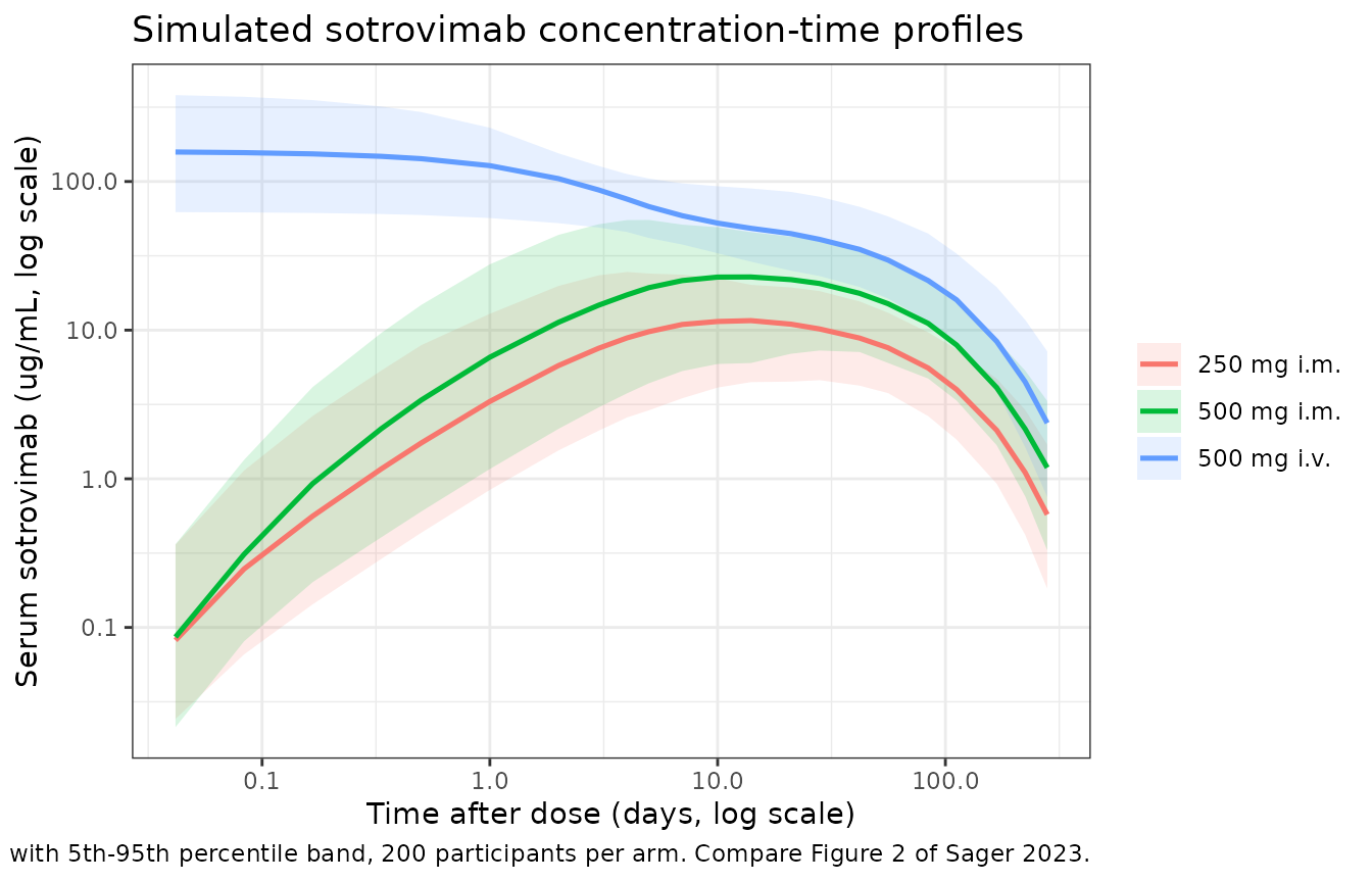
The i.m. arms rise to a broad peak around a week rather than showing
a distinct absorption peak: with KA = 0.00643 1/h the
absorption half-life is 108 h, far slower than distribution and only
modestly faster than the 61-day terminal elimination. That
flip-flop-adjacent behaviour is exactly what the authors’ “sigmoid
absorption model” was introduced to describe.
The zero-order input applies bioavailability to the amount, not the rate
MODEL CODE S1 sets F1 = FIM and
R1 = 130 mg/h on the depot. In NONMEM’s modelled-RATE
convention the infusion duration is amt * F / R1, so the
total amount delivered is amt * F and the rate is fixed.
Getting this backwards – delivering the full amt at rate
R1 – would inflate i.m. exposure by 1/F, about 1.7-fold,
and is a silent failure because the profile shape barely changes. It is
therefore checked explicitly.
typ <- rxode2::zeroRe(mod_pk)
ev  <- rxode2::et(amt = 500, cmt = "depot", rate = -1) |>
  rxode2::et(seq(0, 6, by = 0.05), cmt = "depot") |>
  as.data.frame() |>
  dplyr::mutate(WT = 83.6, BMI = 30.41, SEXF = 0)

dep <- rxode2::rxSolve(typ, ev, addDosing = FALSE, returnType = "data.frame")
#> ℹ omega/sigma items treated as zero: 'etalcl', 'etalvc', 'etalvp', 'etalka', 'etalogitfdepot'

f_male       <- 0.582
expected_dur <- 500 * f_male / 130           # 2.238 h
peak_obs     <- max(dep$depot)

stopifnot(
  # Total delivered is amt * F (291 mg), less the small amount KA removes
  # during the 2.24 h input window -- not the full 500 mg.
  peak_obs < 500 * f_male,
  peak_obs > 500 * f_male * 0.985,
  # The peak lands at the end of the F-scaled input window, not at
  # 500/130 = 3.85 h, which is where an unscaled input would peak.
  abs(dep$time[which.max(dep$depot)] - expected_dur) < 0.06,
  # After the input, the depot must decay at exactly KA.
  abs(dep$depot[which.min(abs(dep$time - 6))] /
        dep$depot[which.min(abs(dep$time - 2.25))] -
        exp(-0.00643 * 3.75)) < 1e-3
)
c(expected_duration_h = round(expected_dur, 3),
  observed_peak_mg    = round(peak_obs, 2),
  amt_times_F_mg      = 500 * f_male)
#> expected_duration_h    observed_peak_mg      amt_times_F_mg
#>               2.238             288.890             291.000
Bioavailability by sex
fim_typ <- rxode2::rxSolve(
  rxode2::zeroRe(mod_pk),
  data.frame(id = 1:2, time = 0, WT = 83.6, BMI = 30.41, SEXF = c(0, 1)),
  addDosing = FALSE, returnType = "data.frame"
)
#> ℹ omega/sigma items treated as zero: 'etalcl', 'etalvc', 'etalvp', 'etalka', 'etalogitfdepot'
#> Warning: multi-subject simulation without without 'omega'
stopifnot(
  abs(fim_typ$fdepot[fim_typ$SEXF == 0] - 0.582) < 1e-3,
  abs(fim_typ$fdepot[fim_typ$SEXF == 1] - 0.471) < 1e-3
)
knitr::kable(
  data.frame(
    Sex = c("Male", "Female"),
    `Published F_IM` = c(0.582, 0.471),
    `Packaged F_IM` = round(c(fim_typ$fdepot[fim_typ$SEXF == 0],
                              fim_typ$fdepot[fim_typ$SEXF == 1]), 4),
    check.names = FALSE
  ),
  caption = "Typical i.m. bioavailability by sex (Sager 2023 Results, 'Final model')."
)| Sex | Published F_IM | Packaged F_IM |
|---|---|---|
| Male | 0.582 | 0.5820 |
| Female | 0.471 | 0.4705 |
PKNCA validation
Sager 2023 reports no noncompartmental analysis table, so the reference values available for an NCA comparison are the model-derived terminal half-life of Table S6 and, for the i.v. arm, the Table S6 clearance. Both are genuine published numbers; PKNCA reaches them by a completely independent route (log-linear regression on the simulated terminal phase, and dose divided by AUC), so agreement is informative rather than circular.
nca_conc <- prof |>
  dplyr::filter(!is.na(Cc)) |>
  dplyr::select(id, time, Cc, label)

nca_dose <- prof |>
  dplyr::distinct(id, label, dose) |>
  dplyr::mutate(time = 0)

conc_obj <- PKNCA::PKNCAconc(nca_conc, Cc ~ time | label + id,
                             concu = "ug/mL", timeu = "h")
dose_obj <- PKNCA::PKNCAdose(nca_dose, dose ~ time | label + id,
                             doseu = "mg")

intervals <- data.frame(
  start = 0, end = Inf,
  cmax = TRUE, tmax = TRUE, aucinf.obs = TRUE,
  half.life = TRUE, cl.obs = TRUE
)

nca_res <- PKNCA::pk.nca(
  PKNCA::PKNCAdata(conc_obj, dose_obj, intervals = intervals)
)
# Published references. Half-life is route-independent (Table S6, median
# 61.236 days = 1469.7 h). Clearance from NCA is dose/AUCinf, which
# equals CL only for the i.v. arm; for the i.m. arms it is CL/F, so no
# published reference is asserted there.
published_nca <- tibble::tribble(
  ~label,         ~half.life, ~cl.obs,
  "500 mg i.v.",    1469.7,    0.003958,
  "500 mg i.m.",    1469.7,    NA_real_,
  "250 mg i.m.",    1469.7,    NA_real_
)

cmp <- nlmixr2lib::ncaComparisonTable(
  simulated = nca_res,
  reference = published_nca,
  by        = "label",
  units     = c(half.life = "h", cl.obs = "L/h"),
  tolerance_pct = 20
)

knitr::kable(
  cmp,
  caption = paste(
    "Simulated (PKNCA) versus published NCA-comparable values.",
    "* differs from reference by >20%.",
    "Published half-life is Sager 2023 Table S6 (median 61.236 days);",
    "published clearance is Table S6 (geometric mean 0.095 L/day = 0.00396 L/h)."
  ),
  align = c("l", "l", "r", "r", "r")
)| NCA parameter | label | Reference | Simulated | % diff |
|---|---|---|---|---|
| t½ (h) | 500 mg i.v. | 1470 | 1510 | +2.7% |
| t½ (h) | 500 mg i.m. | 1470 | 1510 | +2.7% |
| t½ (h) | 250 mg i.m. | 1470 | 1480 | +0.6% |
| CL/F (L/h) | 500 mg i.v. | 0.00396 | 0.00402 | +1.5% |
| CL/F (L/h) | 500 mg i.m. | — | 0.00794 | — |
| CL/F (L/h) | 250 mg i.m. | — | 0.00788 | — |
hl <- nca_res$result |>
  dplyr::filter(PPTESTCD == "half.life") |>
  dplyr::group_by(label) |>
  dplyr::summarise(
    n_fit    = sum(!is.na(PPORRES)),
    n_total  = dplyr::n(),
    median_h = stats::median(PPORRES, na.rm = TRUE),
    .groups  = "drop"
  )

stopifnot(
  # Coverage first. `median(..., na.rm = TRUE)` would happily return a
  # confident number computed from three subjects, so assert that PKNCA
  # actually fitted lambda.z for nearly everyone before believing the
  # median. A subject can legitimately fail if it draws a very low KA
  # and peaks late, which is why this is 90% rather than 100%.
  all(hl$n_fit >= 0.9 * hl$n_total),
  # NCA half-life recovers the published 61.2-day terminal half-life on
  # every arm, to within 15%. Gated on the arm MEDIAN, not on any
  # subject's extreme, so it is reproducible across cohorts.
  all(abs(hl$median_h - 1469.7) / 1469.7 < 0.15),
  # NCA clearance on the i.v. arm must recover CL itself (dose/AUCinf
  # with F = 1). This is the check that would catch a wrong volume /
  # clearance unit conversion. The i.m. arms are deliberately excluded:
  # there dose/AUCinf estimates CL/F, not CL.
  {
    clv <- nca_res$result |>
      dplyr::filter(PPTESTCD == "cl.obs", label == "500 mg i.v.")
    abs(stats::median(clv$PPORRES, na.rm = TRUE) - 0.003958) / 0.003958 < 0.15
  }
)
hl
#> # A tibble: 3 × 4
#>   label       n_fit n_total median_h
#>   <chr>       <int>   <int>    <dbl>
#> 1 250 mg i.m.   200     200    1478.
#> 2 500 mg i.m.   200     200    1510.
#> 3 500 mg i.v.   200     200    1509.
Exposure-response
Predicted progression rates by treatment arm (Table S10)
This is the strongest validation in the vignette, because it is a
zero-parameter end-to-end test. Sager 2023 Table S10
reports the distribution of the model-predicted probability of
progression within each COMET-TAIL arm, computed by feeding
population-PK-predicted C(168h) into the exposure-response
model. Reproducing it requires the PK model, the 168 h read-out and the
exposure-response model all to be right simultaneously; nothing is
fitted or adjusted here.
Table S10 was produced with the base exposure-response model of Table S9 (intercept -3.03, slope -0.0255), which carries no risk-factor term – so those are the coefficients used for this comparison, and the final Table 3 model is validated separately below.
set.seed(20260907)
rxode2::rxSetSeed(20260907)

# COMET-TAIL demographics (Table S5 COMET-TAIL column, Table S8):
# median weight 85.0 kg, median BMI 31.0, 45.3% male.
tail_arms <- tibble::tribble(
  ~label,        ~dose, ~route, ~n_published,
  "250 mg i.m.",   250,  "im",   174,
  "500 mg i.m.",   500,  "im",   361,
  "500 mg i.v.",   500,  "iv",   367
)

c168 <- do.call(rbind, lapply(seq_len(nrow(tail_arms)), function(i) {
  cov <- make_cohort(n_arm, 85.0, 31.0, 1 - 0.453, id_offset = i * 10000L)
  solve_arm(mod_pk, cov, tail_arms$dose[i], tail_arms$route[i], 168) |>
    dplyr::filter(time == 168) |>
    dplyr::transmute(id, label = tail_arms$label[i], CONC_SOTRO_168H = Cc)
}))

# Base ER model, Sager 2023 Table S9.
base_int <- -3.03
base_slp <- -0.0255
c168 <- c168 |>
  dplyr::mutate(p_base = 1 / (1 + exp(-(base_int + base_slp * CONC_SOTRO_168H))))

s10_sim <- c168 |>
  dplyr::group_by(label) |>
  dplyr::summarise(mean = mean(p_base), median = stats::median(p_base),
                   .groups = "drop")

# The published "Overall" row pools the three arms at their real sizes,
# so it is reconstructed as a size-weighted mean rather than by simulating
# unequal arms (the 200-per-arm cap applies to every arm).
w <- tail_arms$n_published[match(s10_sim$label, tail_arms$label)]
overall_mean   <- stats::weighted.mean(s10_sim$mean, w)
overall_median <- stats::weighted.mean(s10_sim$median, w)

s10 <- tibble::tribble(
  ~Arm,             ~`Published mean`, ~`Published median`,
  "250 mg i.m.",      0.0340,            0.0337,
  "500 mg i.m.",      0.0267,            0.0266,
  "500 mg i.v.",      0.0120,            0.0111,
  "Overall",          0.0221,            0.0204
) |>
  dplyr::left_join(
    dplyr::bind_rows(
      s10_sim |> dplyr::rename(Arm = label),
      tibble::tibble(Arm = "Overall", mean = overall_mean, median = overall_median)
    ),
    by = "Arm"
  ) |>
  dplyr::rename(`Simulated mean` = mean, `Simulated median` = median) |>
  dplyr::mutate(`% diff (mean)` = 100 * (`Simulated mean` - `Published mean`) /
                  `Published mean`)

stopifnot(
  # Every arm within 20% of the published mean. This is a joint gate on
  # the PK model, the 168 h exposure metric and the ER coefficients.
  all(abs(s10$`% diff (mean)`) < 20),
  # The overall rate is the tightest of the four because arm-level noise
  # averages out; a sign error or a unit error anywhere in the chain
  # would blow it immediately.
  abs(s10$`% diff (mean)`[s10$Arm == "Overall"]) < 12,
  # Rank order must be preserved: more drug, less progression.
  s10$`Simulated mean`[s10$Arm == "250 mg i.m."] >
    s10$`Simulated mean`[s10$Arm == "500 mg i.m."],
  s10$`Simulated mean`[s10$Arm == "500 mg i.m."] >
    s10$`Simulated mean`[s10$Arm == "500 mg i.v."]
)

knitr::kable(
  s10 |> dplyr::mutate(
    dplyr::across(c(`Simulated mean`, `Simulated median`), ~ round(.x, 4)),
    `% diff (mean)` = round(`% diff (mean)`, 1)
  ),
  caption = "Model-predicted probability of COVID-19 progression through day 29, by treatment arm: packaged models versus Sager 2023 Table S10.",
  align = c("l", "r", "r", "r", "r", "r")
)| Arm | Published mean | Published median | Simulated mean | Simulated median | % diff (mean) |
|---|---|---|---|---|---|
| 250 mg i.m. | 0.0340 | 0.0337 | 0.0345 | 0.0351 | 1.4 |
| 500 mg i.m. | 0.0267 | 0.0266 | 0.0261 | 0.0255 | -2.2 |
| 500 mg i.v. | 0.0120 | 0.0111 | 0.0116 | 0.0112 | -3.3 |
| Overall | 0.0221 | 0.0204 | 0.0218 | 0.0215 | -1.3 |
The risk-factor covariate direction
Table 3 gives an intercept of -4.169 and an additive shift of +1.887
for RISKCATN = 1, and Table S8 gives the population split
as 69.8% with one or fewer risk factors and 30.2% with more than one.
The paper never states outright which level RISKCATN = 1
denotes. Three independent lines settle it as “more than one”.
p_ref   <- 1 / (1 + exp(4.169))            # NRISK_GT1 = 0
p_shift <- 1 / (1 + exp(4.169 - 1.887))    # NRISK_GT1 = 1
p_basem <- 1 / (1 + exp(3.03))             # base model, single intercept

# Mixing the two final intercepts over the published split must land near
# the base model's single intercept. Only one assignment of the 69.8% /
# 30.2% weights does.
mix_gt1_is_one <- 0.698 * p_ref   + 0.302 * p_shift
mix_reversed   <- 0.698 * p_shift + 0.302 * p_ref

stopifnot(
  # The shift raises risk, so it must attach to the higher-risk group.
  p_shift > p_ref,
  # The correct assignment sits close to the base model; the reversed one
  # overshoots it by 50%.
  abs(mix_gt1_is_one - p_basem) < abs(mix_reversed - p_basem),
  abs(mix_gt1_is_one - p_basem) / p_basem < 0.20,
  abs(mix_reversed   - p_basem) / p_basem > 0.40
)

knitr::kable(
  data.frame(
    Quantity = c("P(progression) at zero exposure, <=1 risk factor",
                 "P(progression) at zero exposure, >1 risk factors",
                 "Population mix, RISKCATN = 1 means '>1'",
                 "Population mix, reversed coding",
                 "Base model single intercept (Table S9)"),
    Value = round(c(p_ref, p_shift, mix_gt1_is_one, mix_reversed, p_basem), 4)
  ),
  caption = "Only the '>1 risk factors' coding reproduces the base model's zero-exposure progression rate.",
  align = c("l", "r")
)| Quantity | Value |
|---|---|
| P(progression) at zero exposure, <=1 risk factor | 0.0152 |
| P(progression) at zero exposure, >1 risk factors | 0.0926 |
| Population mix, RISKCATN = 1 means ‘>1’ | 0.0386 |
| Population mix, reversed coding | 0.0693 |
| Base model single intercept (Table S9) | 0.0461 |
The final exposure-response model (Table 3) and Figure 4
er_grid <- tidyr::crossing(
  CONC_SOTRO_168H      = seq(0, 120, by = 2),
  NRISK_GT1 = c(0, 1)
) |>
  dplyr::mutate(id = dplyr::row_number(), time = 0)

er_pred <- rxode2::rxSolve(
  mod_er, events = er_grid,
  keep = c("CONC_SOTRO_168H", "NRISK_GT1")
) |>
  as.data.frame() |>
  dplyr::mutate(risk = factor(NRISK_GT1, levels = c(0, 1),
                              labels = c("<=1 risk factor", ">1 risk factors")))

# The packaged model must reproduce Table 3 arithmetic exactly.
chk <- er_pred |> dplyr::filter(CONC_SOTRO_168H == 0)
stopifnot(
  abs(chk$pprog[chk$NRISK_GT1 == 0] - 1 / (1 + exp(4.169))) < 1e-8,
  abs(chk$pprog[chk$NRISK_GT1 == 1] - 1 / (1 + exp(4.169 - 1.887))) < 1e-8,
  # Slope sign: more exposure, less progression.
  all(diff(er_pred$pprog[er_pred$NRISK_GT1 == 0]) < 0)
)

ggplot(er_pred, aes(CONC_SOTRO_168H, pprog, colour = risk)) +
  geom_line(linewidth = 0.9) +
  scale_y_continuous(labels = scales::percent_format(accuracy = 1)) +
  labs(
    x = "Sotrovimab concentration at 168 h (ug/mL)",
    y = "P(progression through day 29)",
    colour = "Number of risk factors",
    title = "Final exposure-response model (Sager 2023 Table 3)",
    caption = "Compare Figure 4 of Sager 2023, which plots the base-model fit against observed proportions."
  ) +
  theme_bw()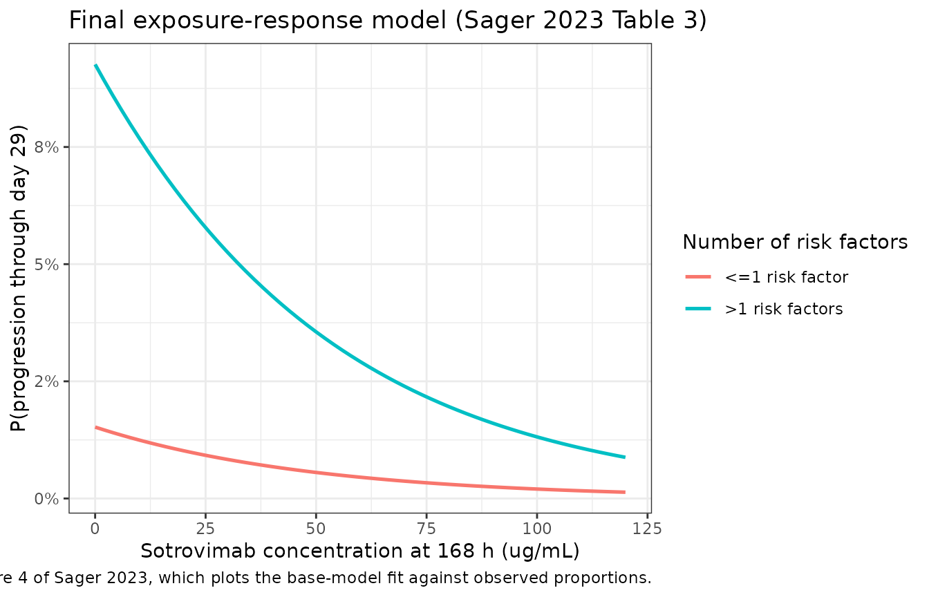
Observed progression rates (Table 2)
Applying the final Table 3 model to the simulated COMET-TAIL cohorts, with the published 30.2% carrying more than one risk factor, should land near the observed 2.2% overall progression rate of Table 2.
set.seed(20260908)

er_cohort <- c168 |>
  dplyr::mutate(NRISK_GT1 = stats::rbinom(dplyr::n(), 1L, 0.302),
                time = 0)

er_final <- rxode2::rxSolve(
  mod_er, events = er_cohort |> dplyr::select(id, time, CONC_SOTRO_168H, NRISK_GT1),
  keep = c("CONC_SOTRO_168H", "NRISK_GT1")
) |>
  as.data.frame() |>
  dplyr::left_join(dplyr::select(er_cohort, id, label), by = "id")

by_arm <- er_final |>
  dplyr::group_by(label) |>
  dplyr::summarise(predicted = mean(pprog), .groups = "drop")

w2 <- tail_arms$n_published[match(by_arm$label, tail_arms$label)]
overall_pred <- stats::weighted.mean(by_arm$predicted, w2)

obs <- tibble::tribble(
  ~label,          ~observed,
  "250 mg i.m.",    0.040,
  "500 mg i.m.",    0.022,
  "500 mg i.v.",    0.014
)

stopifnot(
  # The model-predicted overall rate should sit near the observed 2.2%.
  # The bound is deliberately loose: 20 events in 902 patients carries a
  # binomial standard error of about 0.5 percentage points, so agreement
  # closer than this would be over-claiming.
  abs(overall_pred - 0.022) < 0.010,
  # Rank order across arms must match the observed ordering.
  by_arm$predicted[by_arm$label == "250 mg i.m."] >
    by_arm$predicted[by_arm$label == "500 mg i.v."]
)

knitr::kable(
  by_arm |>
    dplyr::left_join(obs, by = "label") |>
    dplyr::bind_rows(tibble::tibble(label = "Overall",
                                    predicted = overall_pred,
                                    observed = 0.022)) |>
    dplyr::transmute(
      Arm = label,
      `Observed (Table 2)` = observed,
      `Predicted (Table 3 model)` = round(predicted, 4)
    ),
  caption = "Observed versus final-model-predicted progression rates in COMET-TAIL.",
  align = c("l", "r", "r")
)| Arm | Observed (Table 2) | Predicted (Table 3 model) |
|---|---|---|
| 250 mg i.m. | 0.040 | 0.0299 |
| 500 mg i.m. | 0.022 | 0.0240 |
| 500 mg i.v. | 0.014 | 0.0118 |
| Overall | 0.022 | 0.0202 |
The 250 mg i.m. arm is the one the model under-predicts, as the table above shows. That arm contributed 7 events in 174 patients, so its observed 4.0% carries a 95% confidence interval of roughly 1.6% to 8.1% – the model prediction sits comfortably inside it, and the gap is not evidence of a transcription error. Sager 2023 makes the same observation about the C(96h) model in Table S11, where the under-prediction of this arm was severe enough to be the stated reason for preferring C(168h).
Two labelling notes on the PKNCA table above.
ncaComparisonTable() renders cl.obs with the
generic label “CL/F”; on the i.v. arm, where bioavailability is 1 by
construction, that column is CL itself, which is why it is the only arm
carrying a published reference. And the two i.m. arms return the same
CL/F, as they must – clearance and bioavailability are both
dose-independent in this model, so the 250 mg and 500 mg i.m. arms
differ only in scale.
Assumptions and deviations
Original data are not public. All cohorts are virtual, with covariate distributions built to match Sager 2023 Table S5 (population PK) and Tables S5/S8 (COMET-TAIL). Weight and BMI are drawn independently as log-normals matching the published medians; the source does not report their correlation. Only clearance and the peripheral volume depend on weight, and only the absorption rate depends on BMI, so the marginal distributions are what matter for every quantity gated here.
KAunits. Table 1 and the Results text print0.00643 L/h. The packaged model uses 1/h, perMODEL CODE S1 $THETA(;--th5- KA: ... (1/h)) and$DES(DADT(1) = -KA * A(1)). This is a typographical error in the article, corrected from the article’s own supplement.Table 1 footnote b. The printed inverse logit
exp(LFIM)/(1 - exp(LFIM))is a sign error;MODEL CODE S1usesEXP(LFIM)/(1 + EXP(LFIM)), which is what the packaged model implements and what reproduces the 0.471 female bioavailability quoted in the Results.The
F_IMrandom-effect variance is back-solved, not printed. Table 1 givesF_IM’s variability as “42.9 %CV”, but footnote a discloses that this is a delta-method transformation onto the bioavailability scale rather than a log-normal CV, andF_IM’s eta lives on the logit scale. The variance used here (1.0291, i.e. an omega of 1.0144) is recovered from the four printed covariance/correlation pairs involvingF_IM, which agree to within 0.3% of each other. Footnote a’s rounded “1.03” would instead imply an omega of 1.0263 and misses each printed correlation by about 1.2%, so the covariance block is used as the more reliable route. Theomega-checkchunk above verifies that all ten published correlations are reproduced.The i.v. infusion duration is assumed to be 30 minutes. Neither the article nor the supplement states it; Table S1 records only “end of infusion” sampling times. 30 minutes is the sotrovimab labelling. Every quantity gated in this vignette is read at 24 h or later, where the infusion duration is immaterial.
Table S6 spreads are not gated, only central tendency. Table S6 summarises shrunk empirical Bayes estimates (shrinkage 14.6-24.9%, Table 1 footnote n) whereas the simulation applies the full estimated IIV, so simulated geometric CVs are systematically higher. Comparing the spreads would be comparing two different quantities.
Table S10 is reproduced with the base exposure-response model. Table S10 was generated from the Table S9 base model (intercept -3.03, slope -0.0255), which has no risk-factor term. The packaged model is the final model of Table 3, validated separately against Table 3 arithmetic and the Table 2 observed rates. The base coefficients appear only as literals inside the Table S10 comparison chunk and are not packaged as a model.
The published “Overall” rows are reconstructed as size-weighted means. The 200-participants-per-arm cap applies to every arm, so the real 367 / 361 / 174 arm sizes are applied as weights rather than simulated directly.
The C(96h) exposure-response model is not packaged. Sager 2023 fitted it (Table S9,
MODEL CODE S3) but rejected it: Table S11 shows it under-predicts the observed progression rate in the 250 mg i.m. arm. It is an intermediate model, not a final one, so per the package’s replicate-the-authors’ -structure policy only the final C(168h) model is shipped.Convention-checker warnings on the exposure-response model.
checkModelConventions()flagsprogas a non-canonical observation variable andrx.prog.binomas a non-canonical residual-error parameter. Both are artefacts of encoding a Bernoulli endpoint with~ dbinom(1, p); the already-registeredKemal_2026_nemtabrutinib_ae,Kemal_2026_nemtabrutinib_borandRiggs_2012_albinterferon_svr_gt1models produce the identical pair. There is no residual-error parameter to name – the Bernoulli likelihood is the entire error model.Qhas no interindividual variability. Table 1 reports its magnitude of variability as “NE” andMODEL CODE S1writesQ = TVQwith noEXP(ETA(.))factor. The packaged model matches.Generalizability, per the authors. COMET-TAIL had no placebo arm, contributed only 20 progressors, and enrolled during a delta-predominant period (88.2% of sequenced participants). Sager 2023 states explicitly that these limitations may prevent the exposure-response relationship from generalizing across SARS-CoV-2 variants. The
logitprogintercept is described as a “model-estimated placebo response” but is an extrapolation to zero exposure, not an observed placebo rate; the authors note that real-world evidence suggests roughly 9.1% progression in unvaccinated individuals in Florida during the delta period, against the model’s 1.5% at zero exposure for the lower-risk stratum.