Lobaplatin (Cheng 2019)
Source:vignettes/articles/Cheng_2019_lobaplatin.Rmd
Cheng_2019_lobaplatin.RmdModel and source
- Citation: Cheng Y, Wu L, Liu X, Zhao Y, Liu C, Chen Q, Sun T, Zheng Q (2019). Population pharmacokinetics and individualized lobaplatin regimen for the treatment of Chinese small cell lung cancer in the elderly. Medicine (Baltimore) 98(3):e14136. doi:10.1097/MD.0000000000014136.
- Description: Two-compartment population PK model for intravenous lobaplatin in elderly (>= 65 years) Chinese patients with small cell lung cancer (Cheng 2019; n = 113 patients across 7 centres, 678 plasma concentrations). Linear disposition with a small elimination clearance (0.478 L/h) and a long terminal phase. The central volume is an ADDITIVE linear function of body surface area (51.4 L, plus 47.7 L per m^2 above the 1.675 m^2 cohort median), and the inter-compartmental clearance is 31% higher in patients with creatinine clearance >= 80 mL/min. Exponential inter-individual variability on all four disposition parameters and a proportional residual error. IMPORTANT: Cheng 2019 Table 3 labels the two clearances CL1 (0.478 L/h) and CL2 (12.1 L/h) without saying which is elimination and which is distribution, and the Discussion reads CL2 as the renally relevant clearance. The paper’s own published AUC simulations and its visual predictive check both identify CL1 as the ELIMINATION clearance and CL2 as the INTER-COMPARTMENTAL clearance; that assignment is what is encoded here and is gated in the validation vignette.
- Article: https://doi.org/10.1097/MD.0000000000014136 (open access, PMC6370119)
No supplementary material, erratum or corrigendum is associated with this article; the model is fully specified by Table 3 plus the covariate equations printed in Results 3.5 and 3.6.
Population
Cheng 2019 is a prospective, single-arm, seven-centre study (ChiCTR-OPN-15006057) in elderly (>= 65 years) Chinese patients with small cell lung cancer, run from June 2014 to July 2016. Patients were allocated by Cockcroft-Gault creatinine clearance: group A (Ccr >= 80 mL/min, n = 51) received lobaplatin 30 mg/m^2 and group B (60 <= Ccr < 80 mL/min, n = 49) received 20 mg/m^2, each combined with etoposide or irinotecan and repeated for up to four cycles. Baseline characteristics (Table 1): median age 68 years (range 66-71), 75 male / 25 female, cohort Ccr 80.3 mL/min, 30 limited-stage and 70 extensive-stage patients, ECOG 0/1/2 in 11/81/8 patients.
The PK analysis (Results 3.4) pooled 113 patients: the 100 population-study patients, sampled at four random time points in cycle 1 and once at 4 h in later cycles, plus 13 patients at Hunan Cancer Hospital sampled at all ten protocol time points. That gave 678 plasma lobaplatin concentrations, 17 of them below the limit of quantitation. Fifty-six patients received each of the two dose levels. No patient with Ccr < 60 mL/min was enrolled, which the Discussion names as the study’s main limitation.
The same information is available programmatically via
readModelDb("Cheng_2019_lobaplatin")()$population.
Source trace
| Equation / parameter | Value | Source location |
|---|---|---|
lvc (V1) |
51.4 L | Table 3, row V1, L (SE 5.1%; bootstrap 51.5,
46.3-57.2) |
lvp (V2) |
202.0 L | Table 3, row V2, L (SE 5.8%; bootstrap 202.8,
177.6-230.4) |
lcl (CL1, elimination) |
0.478 L/h | Table 3, row CL1, L/h (SE 8.3%; bootstrap 0.478,
0.365-0.602) |
lq (CL2, inter-compartmental) |
12.1 L/h | Table 3, row CL2, L/h (SE 5.9%; bootstrap 12.2,
10.5-14.2) |
e_bsa_vc |
47.7 L per m^2 | Table 3, row Theta of the BSA on V1; Results 3.5 and
3.6, V1 = 51.4 + (BSA-1.675) x 47.7
|
e_crcl_q |
1.31 | Table 3, row Theta of CCRG on CL 2; Results 3.5,
CL2 values of 12.10 L/h and 15.85 L/h
|
etalvc |
0.234455 | Table 3, IIV row V 1 , % = 51.4;
log(1 + 0.514^2)
|
etalvp |
0.298684 | Table 3, IIV row V 2 , % = 59.0;
log(1 + 0.590^2)
|
etalcl |
0.480067 | Table 3, IIV row CL 1 , % = 78.5;
log(1 + 0.785^2)
|
etalq |
0.144306 | Table 3, IIV row CL 2 , % = 39.4;
log(1 + 0.394^2)
|
propSd |
sqrt(0.0321) |
Table 3, row Proportional error, % = 3.21, read as
sigma^2 x 100
|
IIV form Pi = PTV x exp(eta_i)
|
n/a | Methods 2.6.2 and Results 3.6,
Inter-individual variability
|
Residual form Cobs = Cpred x (1 + eps)
|
n/a | Results 3.6, Intra-individual variability
|
| Two-compartment disposition | n/a | Methods 2.6.1; Discussion,
in line with a 2-compartment model
|
| BSA centring 1.675 m^2 | n/a | Results 3.5, median value in this study
|
| Ccr threshold 80 mL/min | n/a | Methods 2.2, group A / group B definition |
| 2 h infusion, TIME from start of infusion | n/a | Derived: Methods 2.3 protocol times vs the Figure 2 CWRES-vs-TIME axis |
| AUC window 0-26 h | n/a | Derived: reproduces the Figure 4 median AUC values; the figure spans 0-26 h |
# Closed-form two-compartment disposition after a constant-rate infusion. Used
# as an independent reference for the packaged model, and to evaluate candidate
# parameter assignments without solving anything.
cc_2cmt_inf <- function(t, dose, tinf, V1, V2, CL, Q) {
  k10 <- CL / V1
  k12 <- Q / V1
  k21 <- Q / V2
  s <- k10 + k12 + k21
  d <- sqrt(s^2 - 4 * k10 * k21)
  alpha <- (s + d) / 2
  beta <- (s - d) / 2
  A <- (alpha - k21) / (V1 * (alpha - beta))
  B <- (k21 - beta) / (V1 * (alpha - beta))
  rate <- dose / tinf
  te <- pmin(t, tinf)
  tp <- pmax(t - tinf, 0)
  rate * A / alpha * (1 - exp(-alpha * te)) * exp(-alpha * tp) +
    rate * B / beta * (1 - exp(-beta * te)) * exp(-beta * tp)
}

auc_2cmt_inf <- function(upper, dose, tinf, V1, V2, CL, Q) {
  stats::integrate(
    function(u) cc_2cmt_inf(u, dose, tinf, V1, V2, CL, Q),
    lower = 0, upper = upper, subdivisions = 4000, rel.tol = 1e-10
  )$value
}

# Table 3 typical values. V1 is quoted at the 1.675 m^2 BSA centring value.
V1_ref <- 51.4
V2_ref <- 202.0
cl1_ref <- 0.478
cl2_ref <- 12.1
ccrg_ratio <- 1.31
bsa_med <- 1.675
V1_of <- function(bsa) V1_ref + 47.7 * (bsa - bsa_med)

# Cheng 2019 does not print the infusion duration. It is recovered from the
# Figure 2 CWRES-vs-TIME panel, whose sampling clusters sit at 2, 4, 6, 8, 10,
# 14 and 26 h, while the protocol (Methods 2.3) samples at 0, 2, 4, 6, 8, 12 and
# 24 h after the END of the infusion: every cluster is a protocol time plus
# exactly 2 h, which identifies both a 2 h infusion and a dataset TIME running
# from the start of that infusion.
tinf_h <- 2
# The exposure window of the Figure 4 simulations, likewise not printed: the
# figure panels span 0-26 h, i.e. 24 h after the end of the infusion.
auc_window_h <- 26
Which clearance is which? Identifying CL1 and CL2
Table 3 prints two clearances, CL1 = 0.478 L/h and
CL2 = 12.1 L/h, and never says which is elimination and
which is distribution. The Discussion reads CL2 as the
renally relevant clearance (“patient grouping according to the Ccr
significantly affected CL2”), which would make CL2 the
elimination clearance. Figure 4 settles it: it prints eighteen median
AUC values from the paper’s own simulations, and they are reproduced
only when CL1 is the elimination clearance and
CL2 the inter-compartmental clearance.
# Median AUC values printed in the legends of Cheng 2019 Figure 4. No unit is
# given; the magnitudes identify them as ug*h/L (= ng*h/mL), matching the ng/mL
# axis of Figure 2, so they are converted to mg*h/L here.
#
# Panel A  - fixed absolute dose of 30 x 2.09 = 62.7 mg for every subject.
# Panel B  - legend says "BSA-based administration of 30 mg/m2" for both groups,
#            but its printed numbers are byte-identical to panel C's; see the
#            deviation note at the end of this vignette. They are transcribed
#            once, as the protocol scenario they actually are.
# Panel C  - protocol dosing: group A 30 mg/m2, group B 20 mg/m2.
# Panel D  - adjusted dosing: group A 30 mg/m2, group B 27 mg/m2.
published_fig4 <- tibble::tribble(
  ~panel, ~scenario, ~BSA, ~group, ~dose_mg, ~auc_pub_ug,
  "A", "Fixed 62.7 mg", 2.09, "B", 62.700, 8060.421,
  "A", "Fixed 62.7 mg", 1.675, "B", 62.700, 8916.259,
  "A", "Fixed 62.7 mg", 1.24, "B", 62.700, 9991.227,
  "A", "Fixed 62.7 mg", 2.09, "A", 62.700, 7501.345,
  "A", "Fixed 62.7 mg", 1.675, "A", 62.700, 8262.232,
  "A", "Fixed 62.7 mg", 1.24, "A", 62.700, 9236.093,
  "C", "Protocol 30 / 20 mg/m2", 1.24, "A", 30 * 1.24, 5479.782,
  "C", "Protocol 30 / 20 mg/m2", 1.675, "A", 30 * 1.675, 6621.644,
  "C", "Protocol 30 / 20 mg/m2", 2.09, "A", 30 * 2.09, 7501.345,
  "C", "Protocol 30 / 20 mg/m2", 1.24, "B", 20 * 1.24, 3951.868,
  "C", "Protocol 30 / 20 mg/m2", 1.675, "B", 20 * 1.675, 4763.868,
  "C", "Protocol 30 / 20 mg/m2", 2.09, "B", 20 * 2.09, 5373.607,
  "D", "Adjusted 30 / 27 mg/m2", 1.24, "A", 30 * 1.24, 5479.782,
  "D", "Adjusted 30 / 27 mg/m2", 1.675, "A", 30 * 1.675, 6621.644,
  "D", "Adjusted 30 / 27 mg/m2", 2.09, "A", 30 * 2.09, 7501.345,
  "D", "Adjusted 30 / 27 mg/m2", 1.24, "B", 27 * 1.24, 5335.025,
  "D", "Adjusted 30 / 27 mg/m2", 1.675, "B", 27 * 1.675, 6431.224,
  "D", "Adjusted 30 / 27 mg/m2", 2.09, "B", 27 * 2.09, 7254.379
) |>
  mutate(
    CRCL = ifelse(group == "A", 95, 70),
    auc_pub = auc_pub_ug / 1000
  )

# Internal consistency of the published figure: at BSA 2.09 m^2 the flat 62.7 mg
# dose of panel A IS 30 mg/m^2, so panels A and C/D must print the same value
# for the group-A / 2.09 m^2 cell. They do (7501.345), which confirms both the
# flat-dose level and that all panels share one AUC definition.
stopifnot(
  n_distinct(published_fig4$auc_pub_ug[published_fig4$BSA == 2.09 & published_fig4$group == "A"]) == 1L
)
fig4_readings <- published_fig4 |>
  tidyr::expand_grid(reading = c("CL1 = elimination", "CL2 = elimination")) |>
  rowwise() |>
  mutate(
    auc_model = if (reading == "CL1 = elimination") {
      auc_2cmt_inf(
        auc_window_h, dose_mg, tinf_h, V1_of(BSA), V2_ref,
        cl1_ref, cl2_ref * ifelse(group == "A", ccrg_ratio, 1)
      )
    } else {
      auc_2cmt_inf(
        auc_window_h, dose_mg, tinf_h, V1_of(BSA), V2_ref,
        cl2_ref * ifelse(group == "A", ccrg_ratio, 1), cl1_ref
      )
    },
    pct_diff = (auc_model / auc_pub - 1) * 100
  ) |>
  ungroup()

fig4_readings |>
  group_by(Reading = reading) |>
  summarise(
    `n values` = n(),
    `Median difference (%)` = round(stats::median(pct_diff), 2),
    `Worst difference (%)` = round(pct_diff[which.max(abs(pct_diff))], 1),
    .groups = "drop"
  ) |>
knitr::kable(caption = "All 18 published Figure 4 median AUC values against AUC(0-26 h) under both CL1 / CL2 assignments.")| Reading | n values | Median difference (%) | Worst difference (%) |
|---|---|---|---|
| CL1 = elimination | 18 | 0.75 | 1.5 |
| CL2 = elimination | 18 | -49.47 | -58.4 |
fit_x <- fig4_readings |> filter(reading == "CL1 = elimination")
fit_y <- fig4_readings |> filter(reading == "CL2 = elimination")

stopifnot(
  # Deterministic typical-value comparison against 18 numbers the authors
  # printed, so the bound is tight. Realised worst case 1.5%.
  max(abs(fit_x$pct_diff)) < 3,
  # Mutation control: the competing assignment must FAIL the same gate, so the
  # test above cannot pass vacuously. Realised ~-53% on every value.
  min(abs(fit_y$pct_diff)) > 25
)
fit_x |>
  transmute(
    Panel = panel, Scenario = scenario, `BSA (m2)` = BSA, Group = group,
    `Dose (mg)` = round(dose_mg, 2),
    `Published AUC0-26 (ug*h/L)` = auc_pub_ug,
    `Model AUC0-26 (ug*h/L)` = round(auc_model * 1000, 1),
    `Difference (%)` = round(pct_diff, 2)
  ) |>
knitr::kable(caption = "Cheng 2019 Figure 4 median AUC values reproduced from the packaged model's parameters (CL1 = elimination).")| Panel | Scenario | BSA (m2) | Group | Dose (mg) | Published AUC0-26 (ug*h/L) | Model AUC0-26 (ug*h/L) | Difference (%) |
|---|---|---|---|---|---|---|---|
| A | Fixed 62.7 mg | 2.090 | B | 62.70 | 8060.421 | 8184.9 | 1.54 |
| A | Fixed 62.7 mg | 1.675 | B | 62.70 | 8916.259 | 9000.5 | 0.94 |
| A | Fixed 62.7 mg | 1.240 | B | 62.70 | 9991.227 | 10021.2 | 0.30 |
| A | Fixed 62.7 mg | 2.090 | A | 62.70 | 7501.345 | 7584.3 | 1.11 |
| A | Fixed 62.7 mg | 1.675 | A | 62.70 | 8262.232 | 8307.7 | 0.55 |
| A | Fixed 62.7 mg | 1.240 | A | 62.70 | 9236.093 | 9215.8 | -0.22 |
| C | Protocol 30 / 20 mg/m2 | 1.240 | A | 37.20 | 5479.782 | 5467.8 | -0.22 |
| C | Protocol 30 / 20 mg/m2 | 1.675 | A | 50.25 | 6621.644 | 6658.1 | 0.55 |
| C | Protocol 30 / 20 mg/m2 | 2.090 | A | 62.70 | 7501.345 | 7584.3 | 1.11 |
| C | Protocol 30 / 20 mg/m2 | 1.240 | B | 24.80 | 3951.868 | 3963.7 | 0.30 |
| C | Protocol 30 / 20 mg/m2 | 1.675 | B | 33.50 | 4763.868 | 4808.9 | 0.94 |
| C | Protocol 30 / 20 mg/m2 | 2.090 | B | 41.80 | 5373.607 | 5456.6 | 1.54 |
| D | Adjusted 30 / 27 mg/m2 | 1.240 | A | 37.20 | 5479.782 | 5467.8 | -0.22 |
| D | Adjusted 30 / 27 mg/m2 | 1.675 | A | 50.25 | 6621.644 | 6658.1 | 0.55 |
| D | Adjusted 30 / 27 mg/m2 | 2.090 | A | 62.70 | 7501.345 | 7584.3 | 1.11 |
| D | Adjusted 30 / 27 mg/m2 | 1.240 | B | 33.48 | 5335.025 | 5351.0 | 0.30 |
| D | Adjusted 30 / 27 mg/m2 | 1.675 | B | 45.23 | 6431.224 | 6492.0 | 0.94 |
| D | Adjusted 30 / 27 mg/m2 | 2.090 | B | 56.43 | 7254.379 | 7366.4 | 1.54 |
This also fixes two quantities the paper never prints: the 2 h infusion duration and the 0-26 h AUC window. Shortening the window to 0-24 h biases every value low by 3.7-5.5%, and lengthening it to 0-28 h biases every value high by 5.1-6.8%, so the agreement above is not an artefact of a freely chosen integration limit.
The text claims in Results 3.8.2-3.8.4
The three percentages quoted in the Results follow from the same Figure 4 numbers. Reproducing them pins down how each was computed.
auc_pub_of <- function(scen, grp, bsa) {
  v <- published_fig4$auc_pub_ug[
    published_fig4$scenario == scen & published_fig4$group == grp & published_fig4$BSA == bsa
  ]
  if (length(v) != 1L) stop("no unique published AUC for ", scen, " / group ", grp, " / BSA ", bsa)
  v
}
# The model is linear in dose, so the equal-30 mg/m^2 scenario of Results 3.8.2
# (whose panel is the one whose numbers the figure duplicates) is recovered from
# the adjusted 27 mg/m^2 group-B value by exact dose scaling.
b30 <- auc_pub_of("Adjusted 30 / 27 mg/m2", "B", bsa_med) * 30 / 27
a30 <- auc_pub_of("Adjusted 30 / 27 mg/m2", "A", bsa_med)
b20 <- auc_pub_of("Protocol 30 / 20 mg/m2", "B", bsa_med)
b27 <- auc_pub_of("Adjusted 30 / 27 mg/m2", "B", bsa_med)

text_claims <- tibble::tribble(
  ~Claim, ~Source, ~Published, ~Computed,
  "Group B AUC is 8% higher than group A at an equal 30 mg/m2 dose",
  "Results 3.8.2", 8, (b30 / a30 - 1) * 100,
  "Protocol dosing separates the groups' AUC by 39%",
  "Results 3.8.3 / Abstract", 39, (a30 / b20 - 1) * 100,
  "Group B AUC is only 3% lower than group A at an adjusted 27 mg/m2",
  "Results 3.8.4", -3, (b27 / a30 - 1) * 100
) |>
  mutate(Difference = Computed - Published)

text_claims |>
  mutate(across(c(Computed, Difference), \(x) round(x, 2))) |>
knitr::kable(caption = "Results 3.8.2-3.8.4 recomputed from the published Figure 4 median AUC values at BSA 1.675 m^2.")| Claim | Source | Published | Computed | Difference |
|---|---|---|---|---|
| Group B AUC is 8% higher than group A at an equal 30 mg/m2 dose | Results 3.8.2 | 8 | 7.92 | -0.08 |
| Protocol dosing separates the groups’ AUC by 39% | Results 3.8.3 / Abstract | 39 | 39.00 | 0.00 |
| Group B AUC is only 3% lower than group A at an adjusted 27 mg/m2 | Results 3.8.4 | -3 | -2.88 | 0.12 |
stopifnot(
  # These are arithmetic on the paper's own printed numbers, so they land within
  # a rounding step of the quoted percentages.
  all(abs(text_claims$Difference) < 1)
)
Note the third row: the published “39% lower” for group B is
AUC_A / AUC_B - 1 = 39.0%, not
1 - AUC_B / AUC_A = 28.1%. The two neighbouring claims are
stated in the direct B vs A form, so Results 3.8.3 alone is
expressed relative to group B.
The terminal phase
A 12.1 L/h elimination clearance would empty the plasma long before the last sampling time, and could not produce the accumulation visible in the four-cycle panel of Figure 3.
tail_check <- tibble::tibble(
  `Time (h)` = c(26, 504, 1008),
  `CL1 = elimination (mg/L)` = cc_2cmt_inf(c(26, 504, 1008), 30 * bsa_med, tinf_h, V1_ref, V2_ref, cl1_ref, cl2_ref),
  `CL2 = elimination (mg/L)` = cc_2cmt_inf(c(26, 504, 1008), 30 * bsa_med, tinf_h, V1_ref, V2_ref, cl2_ref, cl1_ref)
)
knitr::kable(tail_check, digits = 5, caption = "Typical single-dose concentration in the terminal phase, group B, BSA 1.675 m^2.")| Time (h) | CL1 = elimination (mg/L) | CL2 = elimination (mg/L) |
|---|---|---|
| 26 | 0.18056 | 0.00252 |
| 504 | 0.07476 | 0.00012 |
| 1008 | 0.02958 | 0.00004 |
stopifnot(
  # Figure 3, 0-26 h panel: observed median ~0.13 mg/L at 26 h, digitised from
  # the published raster, so roughly +/- 20% reading error applies. The gate is
  # wide because the quantity it separates differs ~70-fold between readings.
  abs(tail_check$`CL1 = elimination (mg/L)`[1] / 0.13 - 1) < 0.6,
  tail_check$`CL2 = elimination (mg/L)`[1] < 0.02
)
The terminal half-life implied by CL1 = elimination is
15 days.
The packaged model against the closed form
mod <- readModelDb("Cheng_2019_lobaplatin")
mod_typ <- rxode2::zeroRe(mod)
#> ℹ parameter labels from comments will be replaced by 'label()'
typ_subj <- tidyr::expand_grid(BSA = c(1.24, 1.675, 2.09), CRCL = c(70, 95)) |>
  mutate(
    id = row_number(),
    arm = ifelse(CRCL >= 80, "Group A (Ccr >= 80)", "Group B (Ccr < 80)"),
    dose_mg_m2 = ifelse(CRCL >= 80, 30, 20),
    dose_mg = dose_mg_m2 * BSA
  )

obs_grid <- sort(unique(c(seq(0, 2, by = 0.05), seq(2, 8, by = 0.1), seq(8, 26, by = 0.25))))

build_events <- function(subj, times, dose_times = 0) {
  dosing <- subj |>
    tidyr::expand_grid(time = dose_times) |>
    mutate(amt = dose_mg, evid = 1L, cmt = "central", rate = dose_mg / tinf_h)
  obs <- subj |>
    tidyr::expand_grid(time = times) |>
    mutate(amt = NA_real_, evid = 0L, cmt = "central", rate = 0)
  bind_rows(dosing, obs) |>
    arrange(id, time, desc(evid)) |>
    as.data.frame()
}

typ_events <- build_events(typ_subj, obs_grid)
# `omega = NA` is required: zeroRe() alone is not enough once any stochastic
# rxSolve() has run in the session, because rxode2 retains the previous solve's
# omega and silently re-samples etas. The tight rtol / atol feed the
# closed-form gate below: when rxode2 integrates the ODEs numerically, its
# default rtol of 1e-6 leaves ~1e-6 relative error against the closed form.
typ_sim <- rxode2::rxSolve(
  mod_typ, events = typ_events, omega = NA,
  keep = c("BSA", "CRCL", "arm", "dose_mg"),
  rtol = 1e-10, atol = 1e-12
)
#> Warning: multi-subject simulation without without 'omega'

# Guard that the typical-value solve really is deterministic: subjects sharing
# a BSA must share vc exactly.
stopifnot(
  typ_sim |>
    group_by(BSA) |>
    summarise(n = n_distinct(round(vc, 10)), .groups = "drop") |>
    pull(n) |>
    (\(x) all(x == 1L))()
)
# rxSolve() returns observation records only, so there is no evid column here.
closed <- typ_sim |>
  filter(time > 0) |>
  mutate(
    ref = cc_2cmt_inf(
      time, dose_mg, tinf_h, V1_of(BSA), V2_ref, cl1_ref,
      cl2_ref * ifelse(CRCL >= 80, ccrg_ratio, 1)
    ),
    rel = abs(Cc / ref - 1)
  )

max_rel <- max(closed$rel)
stopifnot(
  # Deterministic comparison of two independent implementations, so the bound
  # is tight. Realised 5.9e-13 when rxode2 solves the cl / vc / q / vp set
  # analytically (linCmt), and 7.6e-11 when it integrates the ODEs numerically
  # at the rtol / atol passed to typ_sim above (1.1e-6 at the default rtol).
  # A bolus instead of a 2 h infusion, a multiplicative instead of
  # additive BSA term, or a swapped CL / Q would each move this by many orders
  # of magnitude.
  max_rel < 1e-7,
  # Structural covariate arithmetic, exactly as Results 3.5 states it.
  isTRUE(all.equal(47.7 * 0.1, 4.77)),
  isTRUE(all.equal(cl2_ref * ccrg_ratio, 15.851)),
  isTRUE(all.equal(round((ccrg_ratio - 1) * 100), 31))
)
cat(sprintf("Maximum relative difference, packaged model vs closed form: %.2e\n", max_rel))
#> Maximum relative difference, packaged model vs closed form: 7.61e-11
PKNCA validation against the published Figure 4 exposures
Cheng 2019 reports no conventional NCA table, so there is nothing to
feed nlmixr2lib::ncaComparisonTable(). PKNCA is used
instead to recompute the exposure metric the paper does publish - median
AUC over the 0-26 h window, Figure 4 - directly from the packaged model
rather than from the closed form used above.
nca_subj <- published_fig4 |>
  distinct(scenario, BSA, group, dose_mg, CRCL) |>
  mutate(
    id = row_number(),
    treatment = paste0(scenario, " | group ", group, " | BSA ", BSA)
  )

nca_grid <- sort(unique(c(
  seq(0, 2, by = 0.05), seq(2, 6, by = 0.05), seq(6, auc_window_h, by = 0.1), auc_window_h
)))
nca_events <- build_events(nca_subj, nca_grid)
nca_sim <- rxode2::rxSolve(
  mod_typ, events = nca_events, omega = NA, keep = c("BSA", "treatment", "dose_mg")
)
#> Warning: multi-subject simulation without without 'omega'

# Use only `!is.na(Cc)`: a `time > 0` or `Cc > 0` filter would drop the
# time-zero row that PKNCA needs to anchor AUC from 0.
sim_nca <- nca_sim |>
  filter(!is.na(Cc)) |>
  select(id, time, Cc, treatment)
sim_nca <- bind_rows(
  sim_nca,
  sim_nca |> distinct(id, treatment) |> mutate(time = 0, Cc = 0)
) |>
  distinct(id, treatment, time, .keep_all = TRUE) |>
  arrange(id, treatment, time)

conc_obj <- PKNCA::PKNCAconc(as.data.frame(sim_nca), Cc ~ time | treatment + id)

# build_events() carries every subject column through, so `treatment` is already
# on the event table and no join is needed.
dose_obj <- PKNCA::PKNCAdose(
  nca_events |> filter(evid == 1) |> select(id, time, amt, treatment) |> as.data.frame(),
  amt ~ time | treatment + id
)

nca_res <- PKNCA::pk.nca(PKNCA::PKNCAdata(
  conc_obj, dose_obj,
  intervals = data.frame(start = 0, end = auc_window_h, cmax = TRUE, tmax = TRUE, auclast = TRUE)
))

nca_tbl <- as.data.frame(nca_res$result) |>
  filter(PPTESTCD %in% c("cmax", "tmax", "auclast")) |>
  select(id, PPTESTCD, PPORRES) |>
  tidyr::pivot_wider(names_from = PPTESTCD, values_from = PPORRES) |>
  left_join(nca_subj, by = "id")
stopifnot(nrow(nca_tbl) == nrow(nca_subj), !anyNA(nca_tbl$auclast))
nca_cmp <- nca_tbl |>
  left_join(
    published_fig4 |> distinct(scenario, BSA, group, auc_pub_ug),
    by = c("scenario", "BSA", "group")
  ) |>
  mutate(pct_diff = (auclast * 1000 / auc_pub_ug - 1) * 100) |>
  arrange(scenario, group, BSA)

nca_cmp |>
  transmute(
    Scenario = scenario, Group = group, `BSA (m2)` = BSA,
    `Cmax (mg/L)` = round(cmax, 3), `Tmax (h)` = tmax,
    `Published AUC0-26 (ug*h/L)` = auc_pub_ug,
    `PKNCA AUC0-26 (ug*h/L)` = round(auclast * 1000, 1),
    `Difference (%)` = round(pct_diff, 2)
  ) |>
knitr::kable(caption = "PKNCA output from the packaged model against every median AUC value printed in Cheng 2019 Figure 4.")| Scenario | Group | BSA (m2) | Cmax (mg/L) | Tmax (h) | Published AUC0-26 (ug*h/L) | PKNCA AUC0-26 (ug*h/L) | Difference (%) |
|---|---|---|---|---|---|---|---|
| Adjusted 30 / 27 mg/m2 | A | 1.240 | 0.766 | 2 | 5479.782 | 5467.7 | -0.22 |
| Adjusted 30 / 27 mg/m2 | A | 1.675 | 0.735 | 2 | 6621.644 | 6658.1 | 0.55 |
| Adjusted 30 / 27 mg/m2 | A | 2.090 | 0.714 | 2 | 7501.345 | 7584.3 | 1.11 |
| Adjusted 30 / 27 mg/m2 | B | 1.240 | 0.756 | 2 | 5335.025 | 5351.0 | 0.30 |
| Adjusted 30 / 27 mg/m2 | B | 1.675 | 0.702 | 2 | 6431.224 | 6492.0 | 0.94 |
| Adjusted 30 / 27 mg/m2 | B | 2.090 | 0.672 | 2 | 7254.379 | 7366.4 | 1.54 |
| Fixed 62.7 mg | A | 1.240 | 1.291 | 2 | 9236.093 | 9215.8 | -0.22 |
| Fixed 62.7 mg | A | 1.675 | 0.917 | 2 | 8262.232 | 8307.7 | 0.55 |
| Fixed 62.7 mg | A | 2.090 | 0.714 | 2 | 7501.345 | 7584.3 | 1.11 |
| Fixed 62.7 mg | B | 1.240 | 1.417 | 2 | 9991.227 | 10021.1 | 0.30 |
| Fixed 62.7 mg | B | 1.675 | 0.973 | 2 | 8916.259 | 9000.5 | 0.94 |
| Fixed 62.7 mg | B | 2.090 | 0.747 | 2 | 8060.421 | 8184.9 | 1.54 |
| Protocol 30 / 20 mg/m2 | A | 1.240 | 0.766 | 2 | 5479.782 | 5467.7 | -0.22 |
| Protocol 30 / 20 mg/m2 | A | 1.675 | 0.735 | 2 | 6621.644 | 6658.1 | 0.55 |
| Protocol 30 / 20 mg/m2 | A | 2.090 | 0.714 | 2 | 7501.345 | 7584.3 | 1.11 |
| Protocol 30 / 20 mg/m2 | B | 1.240 | 0.560 | 2 | 3951.868 | 3963.7 | 0.30 |
| Protocol 30 / 20 mg/m2 | B | 1.675 | 0.520 | 2 | 4763.868 | 4808.9 | 0.94 |
| Protocol 30 / 20 mg/m2 | B | 2.090 | 0.498 | 2 | 5373.607 | 5456.6 | 1.54 |
stopifnot(
  # Typical-value solve plus trapezoidal integration on a dense grid, so the
  # only slack over the closed-form comparison above is quadrature error.
  max(abs(nca_cmp$pct_diff)) < 3,
  # Tmax must sit at the end of the infusion for a constant-rate input into a
  # linear model. This is what distinguishes an infusion from a bolus, which
  # the AUC comparison alone would not catch.
  all(nca_cmp$tmax == tinf_h)
)
Virtual cohort
Original observed data are not available. The cohort below matches the published design: two arms of 200 patients each, dosed by the protocol (group A 30 mg/m^2, group B 20 mg/m^2). Body surface area is drawn to span the reported 1.24-2.09 m^2 range about the 1.675 m^2 median; creatinine clearance is drawn uniformly inside each group’s enrolment band (the paper reports only the cohort mean of 80.3 mL/min and the group boundaries).
# set.seed() seeds R's RNG for the covariate draws. It does NOT seed rxode2's
# eta sampler, whose streams are partitioned per solver thread, so the etas
# differ between a 2-thread CI runner and a 16-thread workstation. Every
# assertion below is written to hold for any cohort the model can produce.
set.seed(20190103)
n_arm <- 200

make_arm <- function(n, dose_mg_m2, crcl_lo, crcl_hi, arm, id_offset) {
  tibble::tibble(
    id = id_offset + seq_len(n),
    BSA = pmin(pmax(stats::rnorm(n, bsa_med, 0.17), 1.24), 2.09),
    CRCL = stats::runif(n, crcl_lo, crcl_hi),
    arm = arm,
    dose_mg_m2 = dose_mg_m2
  ) |>
    mutate(dose_mg = dose_mg_m2 * BSA)
}

cohort <- bind_rows(
  make_arm(n_arm, 20, 60, 80, "Group B (Ccr < 80)", 0L),
  make_arm(n_arm, 30, 80, 130, "Group A (Ccr >= 80)", n_arm)
)
stopifnot(!anyDuplicated(cohort$id))

vpc_times <- sort(unique(c(0, 0.2, 0.5, 1, 1.5, seq(2, 26, by = 0.5))))
sim <- rxode2::rxSolve(
  mod, events = build_events(cohort, vpc_times), keep = c("BSA", "CRCL", "arm", "dose_mg")
)
#> ℹ parameter labels from comments will be replaced by 'label()'
stopifnot(nrow(sim) > 0, all(sim$Cc >= 0, na.rm = TRUE))
Replicate published figures
# Replicates the 0-26 h panel of Figure 3 of Cheng 2019: median and 2.5th /
# 97.5th percentiles of simulated plasma lobaplatin concentration, pooled over
# the two protocol dose arms as the published panel is.
vpc <- sim |>
  filter(time > 0) |>
  group_by(time) |>
  summarise(
    Q025 = quantile(Cc, 0.025), Q50 = quantile(Cc, 0.50),
    Q975 = quantile(Cc, 0.975), .groups = "drop"
  )

# Digitised from the published 0-26 h panel of Figure 3 (observed median and
# 2.5th / 97.5th percentile lines). Figure-reading error of roughly +/- 15%
# applies to every value; only the median enters a gate.
published_vpc <- tibble::tribble(
  ~time, ~obs_lo, ~obs_med, ~obs_hi,
  2, 0.28, 0.710, 1.47,
  4, 0.17, 0.330, 0.70,
  6, 0.13, 0.260, 0.60,
  8, 0.11, 0.210, 0.48,
  10, 0.095, 0.165, 0.40,
  14, 0.08, 0.140, 0.33,
  26, 0.06, 0.125, 0.29
)

ggplot(vpc, aes(time, Q50)) +
  geom_ribbon(aes(ymin = Q025, ymax = Q975), alpha = 0.25, fill = "steelblue") +
  geom_line(linewidth = 0.9) +
  geom_pointrange(
    data = published_vpc, aes(x = time, y = obs_med, ymin = obs_lo, ymax = obs_hi),
    colour = "darkorange", inherit.aes = FALSE
  ) +
  scale_y_log10() +
  labs(
    x = "Time from start of infusion (h)", y = "Plasma lobaplatin (mg/L)",
    title = "Figure 3 (0-26 h panel): simulated VPC vs digitised published percentiles",
    caption = paste(
      "Line and band: simulated median with 2.5th-97.5th percentiles, n =", 2 * n_arm,
      "| points: median and 2.5th / 97.5th percentiles digitised from Cheng 2019 Figure 3."
    )
  )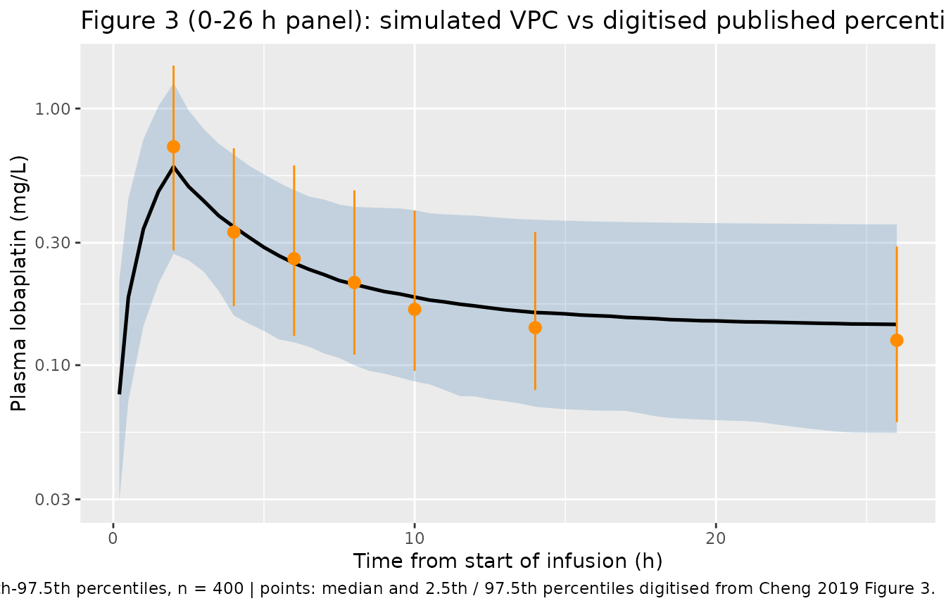
vpc_cmp <- published_vpc |>
  left_join(vpc, by = "time") |>
  mutate(pct_diff = (Q50 / obs_med - 1) * 100)
stopifnot(nrow(vpc_cmp) == nrow(published_vpc), !anyNA(vpc_cmp$pct_diff))

vpc_cmp |>
  transmute(
    `Time (h)` = time, `Published median (mg/L)` = obs_med,
    `Simulated median (mg/L)` = round(Q50, 3), `Difference (%)` = round(pct_diff, 1)
  ) |>
knitr::kable(caption = "Simulated cohort median against the digitised Figure 3 median.")| Time (h) | Published median (mg/L) | Simulated median (mg/L) | Difference (%) |
|---|---|---|---|
| 2 | 0.710 | 0.593 | -16.4 |
| 4 | 0.330 | 0.346 | 4.8 |
| 6 | 0.260 | 0.250 | -4.0 |
| 8 | 0.210 | 0.207 | -1.6 |
| 10 | 0.165 | 0.184 | 11.6 |
| 14 | 0.140 | 0.160 | 14.6 |
| 26 | 0.125 | 0.144 | 15.3 |
stopifnot(
  # Assert on the CENTRE of the distribution, never on its extremes: the tails
  # of a random cohort are not reproducible across rxode2 builds or solver
  # thread counts. The median of 400 subjects is stable to a few percent; the
  # remaining tolerance covers digitisation error on the published raster.
  abs(stats::median(vpc_cmp$pct_diff)) < 30,
  stats::quantile(abs(vpc_cmp$pct_diff), 0.9) < 45
)
# Replicates the four-cycle panel of Figure 3: accumulation over four 21-day
# cycles. The cycle length is not printed; it is taken from the ~1500 h span of
# the published panel, which is three inter-dose intervals of ~504 h.
cycle_h <- 21 * 24
cycle_sim <- rxode2::rxSolve(
  mod_typ,
  events = build_events(
    typ_subj,
    times = sort(unique(c(seq(0, 4 * cycle_h, by = 6), cycle_h * (0:3) + 4))),
    dose_times = cycle_h * (0:3)
  ),
  omega = NA, keep = c("BSA", "arm")
)
#> Warning: multi-subject simulation without without 'omega'

cycle_sim |>
  filter(BSA == bsa_med) |>
  ggplot(aes(time / 24, Cc, colour = arm)) +
  geom_line() +
  labs(
    x = "Time (days)", y = "Plasma lobaplatin (mg/L)", colour = NULL,
    title = "Figure 3 (four-cycle panel): typical-value profile, BSA 1.675 m^2",
    caption = "Replicates the four-cycle panel of Figure 3 of Cheng 2019."
  )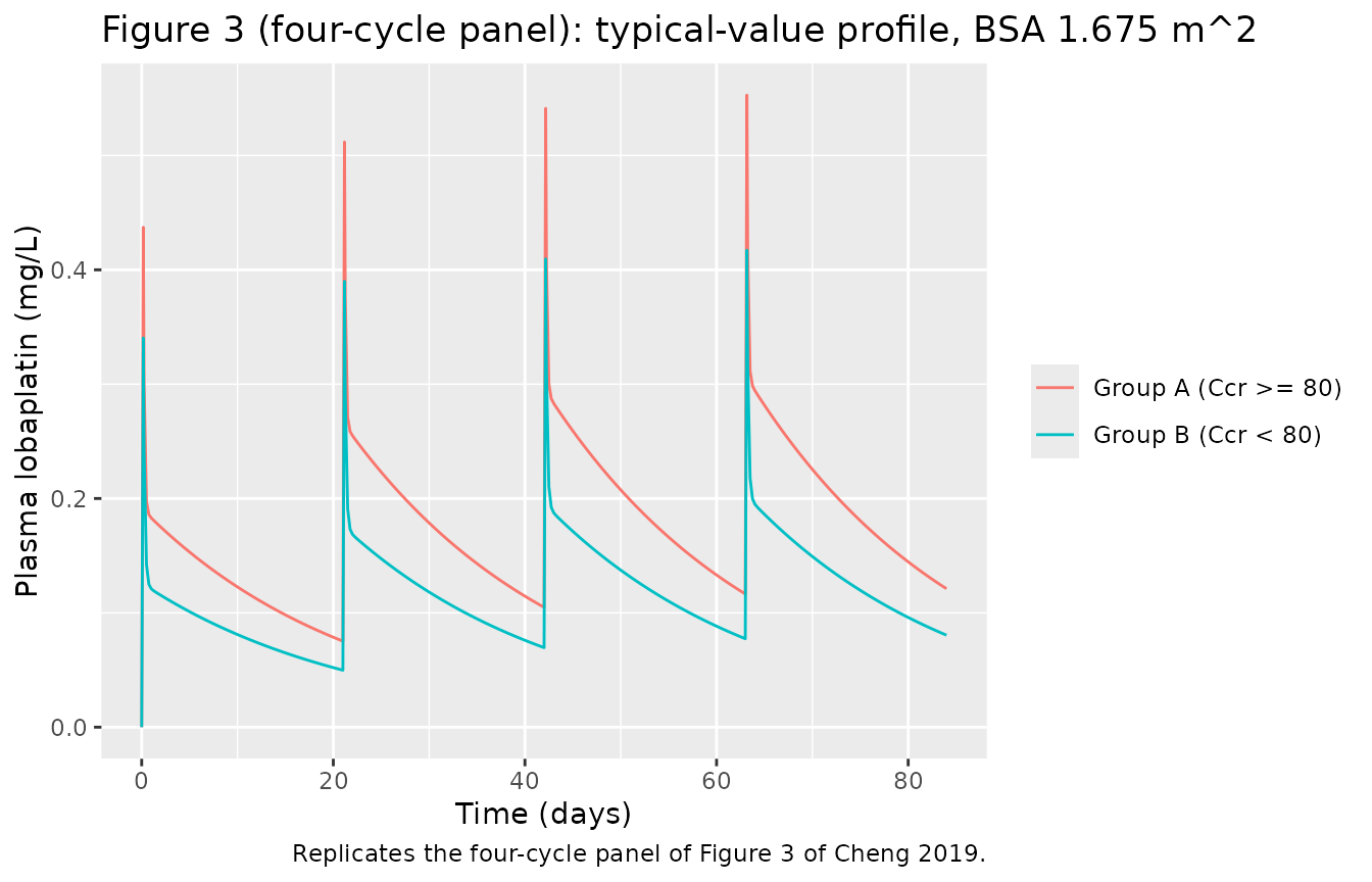
# Concentration 4 h after each cycle's dose, the sampling time the published
# four-cycle panel plots for cycles 2-4.
cyc_a <- cycle_sim |> filter(BSA == bsa_med, arm == "Group A (Ccr >= 80)")
c4h <- vapply(cycle_h * (0:3) + 4, function(tt) {
  v <- cyc_a$Cc[abs(cyc_a$time - tt) < 1e-6]
  if (length(v) != 1L) stop("no unique 4 h post-dose row at t = ", tt)
  v
}, numeric(1))

stopifnot(
  # Deterministic typical-value quantities, so exact ordering is safe here.
  length(c4h) == 4L, all(diff(c4h) > 0),
  # The published panel shows the 4 h points rising across the four cycles.
  c4h[4] / c4h[1] > 1.1, c4h[4] / c4h[1] < 1.6
)
cat(sprintf("Accumulation ratio (4 h post-dose, cycle 4 / cycle 1): %.2f\n", c4h[4] / c4h[1]))
#> Accumulation ratio (4 h post-dose, cycle 4 / cycle 1): 1.26
Does body-surface-area dosing reduce exposure variability?
Cheng 2019’s clinical conclusion is that “with Ccr >= 60 ml/min, BSA based administration is necessary”. The model does not support it, and neither do the paper’s own Figure 4 numbers. This is reported as a deviation rather than gated.
spread <- function(x) max(x) / min(x)

bsa_dosing <- published_fig4 |>
  filter(group == "A") |>
  mutate(regimen = ifelse(scenario == "Fixed 62.7 mg", "Fixed 62.7 mg", "BSA-based 30 mg/m2")) |>
  distinct(regimen, BSA, auc_pub_ug) |>
  group_by(regimen) |>
  summarise(
    `Lowest AUC0-26 (ug*h/L)` = min(auc_pub_ug),
    `Highest AUC0-26 (ug*h/L)` = max(auc_pub_ug),
    `Spread (fold)` = round(spread(auc_pub_ug), 3),
    .groups = "drop"
  )

model_spread <- c(
  `Fixed 62.7 mg` = spread(vapply(
    c(1.24, 1.675, 2.09),
    \(b) auc_2cmt_inf(auc_window_h, 62.7, tinf_h, V1_of(b), V2_ref, cl1_ref, cl2_ref * ccrg_ratio),
    numeric(1)
  )),
  `BSA-based 30 mg/m2` = spread(vapply(
    c(1.24, 1.675, 2.09),
    \(b) auc_2cmt_inf(auc_window_h, 30 * b, tinf_h, V1_of(b), V2_ref, cl1_ref, cl2_ref * ccrg_ratio),
    numeric(1)
  ))
)

bsa_dosing |>
  mutate(`Model spread (fold)` = round(unname(model_spread[regimen]), 3)) |>
  rename(Regimen = regimen) |>
knitr::kable(caption = "Exposure spread across the cohort BSA range (1.24-2.09 m^2), group A, from the published Figure 4 values and from the packaged model.")| Regimen | Lowest AUC0-26 (ug*h/L) | Highest AUC0-26 (ug*h/L) | Spread (fold) | Model spread (fold) |
|---|---|---|---|---|
| BSA-based 30 mg/m2 | 5479.782 | 7501.345 | 1.369 | 1.387 |
| Fixed 62.7 mg | 7501.345 | 9236.093 | 1.231 | 1.215 |
stopifnot(
  # The model must agree with the paper's OWN printed numbers, which is the
  # gate. That the direction contradicts the paper's conclusion is recorded in
  # the deviations section, not asserted away.
  all(abs(model_spread[bsa_dosing$regimen] / bsa_dosing$`Spread (fold)` - 1) < 0.05)
)
Both the published values and the model give a wider
exposure spread under BSA-based dosing (about 1.37-fold across 1.24-2.09
m^2) than under a flat 62.7 mg dose (about 1.23-fold). The mechanism is
in the covariate model itself: BSA was retained on the central volume
only, never on clearance, and the fitted additive slope is steep enough
that V1 more than doubles (30.7 to 71.2 L) while BSA rises only
1.69-fold. A flat dose is therefore already over-compensated by the
volume increase, and scaling the dose to BSA on top of that
over-corrects. At AUC(0-inf), where exposure is
dose / CL and BSA does not enter at all, a flat dose gives
zero spread and BSA-based dosing gives the full 1.69-fold dose
spread.
Assumptions and deviations
Model-structure interpretation
CL1is the elimination clearance andCL2the inter-compartmental clearance, against the Discussion’s reading ofCL2as the renally relevant clearance. All eighteen median AUC values printed in Figure 4 are reproduced to within 1.5% on that assignment and missed by about 53% on the other, and the gate includes the failing alternative as a mutation control. A consequence worth flagging to anyone reusing the model: creatinine clearance acts on distribution, not on elimination, so its effect on total exposure is small (about 8% over 0-26 h, and nil atAUC(0-inf)) rather than the 31% one would read off the clearance ratio.Results 3.8.3 states its comparison relative to group B. The published “39% lower” for group B under protocol dosing is
AUC_A / AUC_B - 1 = 39.0%, not1 - AUC_B / AUC_A = 28.1%. The two neighbouring claims (3.8.2 and 3.8.4) are in the directB vs Aform and match to within 0.1 percentage points.The paper’s clinical conclusion is not reproducible from its own model. See the section above: both the packaged model and Cheng 2019’s own Figure 4 values show BSA-based dosing widening the exposure spread relative to a flat dose. Results 3.8.1 observes that a flat dose gives different AUCs in different-BSA patients and concludes BSA-based dosing is needed, without comparing the two spreads; Results 3.8.2 describes the BSA-based spread as “small” but prints values ranging 5480 to 7501 across the BSA range. Nothing was tuned to reach this; the model reproduces every published number.
Errors in the published figures
Panels B and C of Figure 4 print identical median AUC values. Panel B is captioned as BSA-based 30 mg/m^2 for both groups and panel C as protocol dosing (30 and 20 mg/m^2), which cannot give the same numbers. The values are the protocol scenario: the group-B entries equal the panel-D 27 mg/m^2 entries scaled by exactly 20/27, which a 30 mg/m^2 arm cannot do. The equal-dose scenario of Results 3.8.2 is therefore not printed anywhere and is recovered here by dose scaling, which is exact because the model is linear.
The two panels of Figure 3 carry transposed sub-captions. The panel labelled “VPC for all 4 cycles” spans 0-26 h and the one labelled “VPC for 0~24 hours” spans 0-1500 h. Section 3.7 also describes the dashed lines as the 5th and 95th percentiles while the figure caption calls them the 2.5th and 97.5th; the caption is used here.
Methods 2.6.2 and Results 3.6 disagree on the residual-error model. Methods 2.6.2 says the proportional-additive model had the lowest OFV but its covariance step failed, “therefore the more stable proportional model was selected”; Results 3.6 opens by saying intra-individual variability “was described by the proportional additive model”. Table 3 lists a single proportional row and no additive row, and the equation printed immediately below in Results 3.6 is proportional only. The proportional-only model is encoded.
Values whose scale the source does not state
Inter-individual variability rows of Table 3 are read as CV% for the exponential IIV model of Methods 2.6.2, converted exactly with
omega^2 = log(1 + CV^2). The competing reading, that the printed number is the raw NONMEM variance multiplied by 100 (omega^2 = 0.514for V1, and so on), is excluded by the 0-26 h panel of Figure 3: simulating the published design under that reading gives a mean log-scale spread of about 0.60 against the 0.38 measured off the published percentile lines, whereas the CV% reading gives 0.44. Table 3 carries no footnote defining the transformation.The residual row of Table 3 is read as
sigma^2 x 100, givingpropSd = sqrt(0.0321) = 17.9%. Taken at face value the row would be a 3.21% proportional error. That is rejected on two grounds: it sits below the +/-15% precision that the CFDA bioanalytical guideline cited in Methods 2.4 allows for the assay itself, and the paper’s own IPRED-vs-OBS panel (Figure 2, upper left) shows scatter about the identity line of roughly 13-18% at every prediction level, which a 3.21% error cannot produce. This is the one place where the table’s two variability blocks are read on different scales; the evidence for each is independent and is set out above. Neither choice changes any gate in this vignette, all of which are on typical values or on a cohort median.
Values the source does not print at all
The 2 h infusion duration and the 0-26 h AUC window are derived, not printed. The duration comes from the Figure 2 CWRES-vs-TIME axis, on which every sampling cluster is a Methods 2.3 protocol time plus exactly 2 h; the window is identified by the Figure 4 reproduction above, which degrades to -3.7/-5.5% at 0-24 h and +5.1/+6.8% at 0-28 h. Both live in the vignette’s event table, not in the model file.
The cycle length of 21 days is taken from the ~1500 h span of the four-cycle panel of Figure 3 (three inter-dose intervals of about 504 h) and is used only for the accumulation figure.
The unit of the Figure 4 median AUC values is not printed. It is taken as ugh/L (= ngh/mL) from the magnitudes and from the ng/mL axis of Figure 2.
The digitised Figure 3 percentiles were read off the published raster by the maintainers; roughly +/- 15% reading error applies and that section’s gate is set accordingly.
Cohort assumptions
- Body surface area is drawn as a normal distribution centred on the published median of 1.675 m^2 and truncated to the published 1.24-2.09 m^2 range; the paper reports only those three values, not the shape.
- Creatinine clearance is drawn uniformly within each group’s enrolment band (60-80 and 80-130 mL/min). Only the 80 mL/min threshold affects the model, so the within-band shape is immaterial to every result here.
- Co-administered etoposide or irinotecan is not modelled: Results 3.5 reports that chemotherapy regimen was screened as a covariate and not retained.
Not modelled
- The title and Introduction promise a population PK and PD analysis, and motivate it with the reported correlation between thrombocytopenia score and free-platinum AUC. No PD model, PD parameter table or exposure-response equation appears anywhere in the article; Section 3 reports adverse-event incidences only (Table 2). There is therefore no PD layer to extract, and none is encoded.
- The separate whole-blood total-platinum assay described in Methods 2.3 has no reported model or parameters; only the plasma lobaplatin analysis is encoded.