Piperacillin (Bulitta 2010)
Source:vignettes/articles/Bulitta_2010_piperacillin.Rmd
Bulitta_2010_piperacillin.RmdModel and source
- Citation: Bulitta JB, Kinzig M, Jakob V, Holzgrabe U, Sorgel F, Holford NHG. Nonlinear pharmacokinetics of piperacillin in healthy volunteers – implications for optimal dosage regimens. Br J Clin Pharmacol. 2010;70(5):682-693. doi:10.1111/j.1365-2125.2010.03750.x
- Description: Three-compartment population PK model for piperacillin in healthy adult volunteers after a single intravenous infusion, with first-order non-renal clearance and parallel first-order plus mixed-order (Michaelis-Menten) renal elimination, allometrically scaled to 70 kg; a urine compartment accumulates the renally excreted amount (Bulitta 2010 Model 3, final model, NONMEM estimates)
- Article: https://doi.org/10.1111/j.1365-2125.2010.03750.x
Population
The Bulitta 2010 study was a single-centre, open-label, five-period replicate-dose trial in 4 healthy Caucasian adult volunteers (2 male, 2 female; ages 22 to 24 years; weights 67 to 85 kg with median 77.5 kg; heights 164 to 178 cm; Table 1). Each subject received a single 4 g intravenous 5-minute infusion of piperacillin on each of five separate study days (occasions on days 1, 3, 10, 24, and 52), so the dataset comprised 20 effective profiles (4 subjects times 5 occasions) used for the population PK analysis. Plasma sampling ran from end-of-infusion to 24 h, and complete urine collection spanned the same window split into 9 intervals (Methods, Sampling schedule). Piperacillin was given alone (no tazobactam).
The same information is available programmatically via the model’s
population metadata
(readModelDb("Bulitta_2010_piperacillin")$population).
Source trace
The per-parameter origin is recorded as an in-file comment next to
each ini() entry in
inst/modeldb/specificDrugs/Bulitta_2010_piperacillin.R. The
table below collects them in one place for review. All parameters are
taken from the NONMEM (FOCE+I) column of Table 3; the paper notes that
the NONMEM estimates were used for the Monte Carlo simulations and that
they had slightly better predictive performance than the S-ADAPT
estimates.
| Equation / parameter | Value | Source location |
|---|---|---|
lcl_nonren (CL_NR for 70 kg, L/h) |
log(4.40) | Table 3 column NONMEM |
lcl_renal (CL_R for 70 kg, L/h) |
log(5.70) | Table 3 column NONMEM |
lvmax (V_max for 70 kg, mg/h) |
log(170) | Table 3 column NONMEM |
lkm (K_m, mg/L) |
log(49.7) | Table 3 column NONMEM |
lvc (V_1 for 70 kg, L) |
log(7.00) | Table 3 column NONMEM |
lvp (V_2 for 70 kg, L) |
log(2.95) | Table 3 column NONMEM |
lvp2 (V_3 for 70 kg, L) |
log(2.71) | Table 3 column NONMEM |
lq (CL_ic_shallow for 70 kg, L/h) |
log(12.7) | Table 3 column NONMEM |
lq2 (CL_ic_deep for 70 kg, L/h) |
log(1.28) | Table 3 column NONMEM |
e_wt_cl (allometric exponent on CL / V_max) |
0.75 fixed | Table 3 footnote * |
e_wt_vc (allometric exponent on volumes) |
1.00 fixed | Table 3 footnote + |
etalcl_renal_nonren (shared CL eta, 9.62% CV) |
0.009211 | Table 3 footnote |
etalvc_vp_vp2 (shared V_ss eta, 13.5% CV) |
0.018061 | Table 3 V_ss row; omega^2 = log(0.135^2 + 1) |
cov(etalcl_renal_nonren,
etalvc_vp_vp2) |
0.010835 | Table 3 footnote ++ (r = 0.84) |
etalvmax (V_max eta, 50.4% CV) |
0.226374 | Table 3 V_max row; omega^2 = log(0.504^2 + 1) |
etalkm (K_m eta, 150% CV) |
1.178655 | Table 3 K_m row; omega^2 = log(1.50^2 + 1) |
cov(etalvmax, etalkm) |
0.511422 | Table 3 footnote SS (r = 0.99) |
propSd (CV_C 12.5%) |
0.125 | Table 3 column NONMEM |
addSd (SD_C 0.447 mg/L) |
0.447 | Table 3 column NONMEM |
propSd_Aurine (CV_AU 24.6%) |
0.246 | Table 3 column NONMEM |
addSd_Aurine (SD_AU 3.89 mg) |
3.89 | Table 3 column NONMEM |
| Three-compartment disposition; parallel first-order plus mixed-order (Michaelis-Menten) renal elimination; first-order non-renal elimination | n/a | Methods ‘Models. Disposition and drug elimination’; Equation 1; Results ‘Model building’ (Model 3 chosen as final) |
| Zero-order infusion duration 5 min | n/a | Methods ‘Study design and drug administration’; study used 5-min IV infusions |
Virtual cohort
The original observed data are not publicly available. The simulation below uses a virtual cohort that approximates the Table 1 demographics: 4 subjects with body weights drawn from a normal distribution centred at the reported weight median (77.5 kg) with a standard deviation tuned so the 67-85 kg range of the four real volunteers is covered. The five replicate occasions within each subject are not simulated separately because the model carries combined between-subject and between-occasion variability in a single PPV term per parameter (Methods, Individual pharmacokinetic model); the within-subject crossover structure is therefore reproduced implicitly through the random effects.
Simulation
Each subject receives a 4 g IV infusion over 5 minutes into the central compartment. The simulations are run on a dense grid out to 24 h so that plasma drug concentrations and the cumulative amount excreted unchanged in urine can be sampled finely and used by PKNCA.
infusion_h <- 5 / 60  # 5 minutes -> hours
dose_mg    <- 4000

obs_times <- sort(unique(c(
  seq(0,  1, by = 0.05),
  seq(1,  6, by = 0.1),
  seq(6, 24, by = 0.25)
)))

make_subject <- function(i, wt) {
  dose_row <- tibble::tibble(
    id   = i,
    time = 0,
    amt  = dose_mg,
    rate = dose_mg / infusion_h,
    evid = 1L,
    cmt  = "central",
    WT   = wt
  )
  obs_rows <- tibble::tibble(
    id   = i,
    time = obs_times,
    amt  = NA_real_,
    rate = NA_real_,
    evid = 0L,
    cmt  = "Cc",
    WT   = wt
  )
  dplyr::bind_rows(dose_row, obs_rows)
}

events <- purrr::map2_dfr(cohort$id, cohort$WT, make_subject) |>
  dplyr::arrange(id, time, dplyr::desc(evid))

stopifnot(!anyDuplicated(unique(events[, c("id", "time", "evid")])))
mod <- readModelDb("Bulitta_2010_piperacillin")
sim <- rxode2::rxSolve(mod, events = events, keep = "WT") |> as.data.frame()
#> ℹ parameter labels from comments will be replaced by 'label()'
The typical-value profile (zero between-subject variability) is also useful for replicating the published mean profiles without stochastic spread:
mod_typical <- mod |> rxode2::zeroRe()
#> ℹ parameter labels from comments will be replaced by 'label()'
sim_typical <- rxode2::rxSolve(mod_typical, events = events, keep = "WT") |>
  as.data.frame()
#> ℹ omega/sigma items treated as zero: 'etalcl_renal_nonren', 'etalvc_vp_vp2', 'etalvmax', 'etalkm'
#> Warning: multi-subject simulation without without 'omega'
Replicate published figures
Figure 1: plasma concentrations and amounts excreted in urine
Bulitta 2010 Figure 1 shows the observed plasma concentrations and the cumulative amounts excreted unchanged in urine after the 4 g 5-minute infusion, overlaid with the median and the 10th-90th percentile envelope of the population predictions. The plots below show the typical-value plasma profile and the cumulative urine amount from the packaged model for the four virtual subjects.
sim_typical |>
  dplyr::filter(time > 0, time <= 12) |>
  ggplot(aes(x = time, y = Cc, group = id, colour = factor(WT))) +
  geom_line(linewidth = 0.7) +
  scale_y_log10() +
  labs(
    x       = "Time after start of infusion (h)",
    y       = "Plasma piperacillin (mg/L)",
    colour  = "Body weight (kg)",
    caption = "Replicates Figure 1 (plasma panels) of Bulitta 2010, typical-value profile."
  ) +
  theme_bw()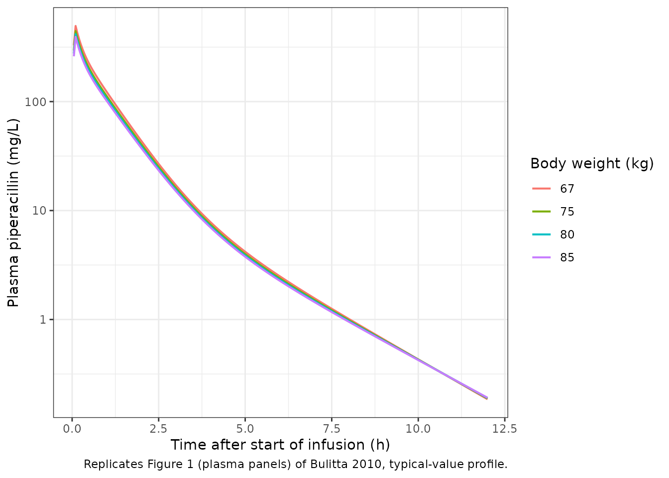
sim_typical |>
  dplyr::filter(time <= 24) |>
  ggplot(aes(x = time, y = Aurine, group = id, colour = factor(WT))) +
  geom_line(linewidth = 0.7) +
  labs(
    x       = "Time after start of infusion (h)",
    y       = "Cumulative piperacillin in urine (mg)",
    colour  = "Body weight (kg)",
    caption = "Replicates Figure 1 (urine panels) of Bulitta 2010, typical-value cumulative urine."
  ) +
  theme_bw()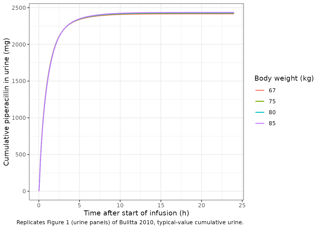
Figure 2: total, renal, and non-renal clearance as a function of plasma concentration
Bulitta 2010 Figure 2 plots renal, non-renal, and total clearance of piperacillin for a typical 70 kg subject against plasma concentration. The non-renal clearance is constant; the renal clearance has a first-order component (constant) and a mixed-order component that decays as the Michaelis-Menten denominator grows with concentration; the total clearance is the sum of the three. Equation 1 of the paper predicts a typical-subject total clearance decreasing from 13.5 L/h at 0 mg/L to 10.8 L/h at 200 mg/L.
c_grid <- seq(0, 300, length.out = 301)

cl_nonren_70 <- 4.40
cl_renal_70  <- 5.70
vmax_70      <- 170
km_val       <- 49.7

clearance <- tibble::tibble(
  concentration_mg_L = c_grid,
  CL_nonrenal        = cl_nonren_70,
  CL_renal_linear    = cl_renal_70,
  CL_renal_saturable = vmax_70 / (km_val + c_grid),
  CL_total           = CL_nonrenal + CL_renal_linear + CL_renal_saturable
)

clearance |>
  tidyr::pivot_longer(
    cols      = c(CL_nonrenal, CL_renal_linear, CL_renal_saturable, CL_total),
    names_to  = "component",
    values_to = "clearance_L_h"
  ) |>
  ggplot(aes(x = concentration_mg_L, y = clearance_L_h, colour = component)) +
  geom_line(linewidth = 0.8) +
  labs(
    x       = "Plasma piperacillin (mg/L)",
    y       = "Clearance (L/h)",
    colour  = "Component",
    caption = "Replicates Figure 2 of Bulitta 2010 for a typical 70 kg subject."
  ) +
  theme_bw()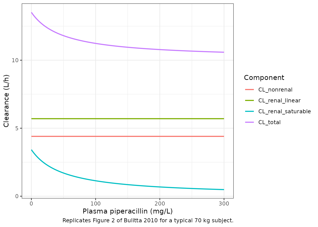
A spot check against the paper’s Equation 1 prediction: total clearance should be 13.5 L/h at 0 mg/L and 10.8 L/h at 200 mg/L.
cl_total_at <- function(c_mgL) {
  cl_nonren_70 + cl_renal_70 + vmax_70 / (km_val + c_mgL)
}
tibble::tibble(
  `Cc (mg/L)`           = c(0, 200),
  `Paper text (L/h)`    = c(13.5, 10.8),
  `Equation 1 (L/h)`    = c(round(cl_total_at(0), 2), round(cl_total_at(200), 2))
) |>
  knitr::kable(digits = 2,
caption = "Bulitta 2010 Equation 1 reproduction at the two concentrations cited in the Results.")| Cc (mg/L) | Paper text (L/h) | Equation 1 (L/h) |
|---|---|---|
| 0 | 13.5 | 13.52 |
| 200 | 10.8 | 10.78 |
PKNCA validation
PKNCA is used to compute Cmax, Tmax, AUC_0-inf, terminal half-life, and total body clearance from the simulated plasma profile. The renal-only clearance and the fraction of dose excreted unchanged in urine are computed by hand from the cumulative urine compartment because PKNCA does not consume cumulative-amount columns directly. The typical-value profile is used so the NCA comparison reflects the published population-mean parameters and is not diluted by the small four-subject sample variability.
sim_nca <- sim_typical |>
  dplyr::filter(!is.na(Cc)) |>
  dplyr::select(id, time, Cc, WT)

# Guarantee a time = 0 row per id (Cc = 0 at pre-infusion).
sim_nca <- dplyr::bind_rows(
  sim_nca,
  sim_nca |> dplyr::distinct(id, WT) |> dplyr::mutate(time = 0, Cc = 0)
) |>
  dplyr::distinct(id, time, .keep_all = TRUE) |>
  dplyr::arrange(id, time)

# Single-treatment cohort -- everyone gets the same 4 g infusion. The PKNCA
# formula uses `treatment + id` as the grouping; we add a single-level
# treatment column so the grouping is well-defined.
sim_nca$treatment <- "4 g IV 5-min"

dose_df <- events |>
  dplyr::filter(evid == 1) |>
  dplyr::select(id, time, amt) |>
  dplyr::mutate(treatment = "4 g IV 5-min")

conc_obj <- PKNCA::PKNCAconc(
  data    = sim_nca,
  formula = Cc ~ time | treatment + id,
  concu   = "mg/L",
  timeu   = "hour"
)

dose_obj <- PKNCA::PKNCAdose(
  data    = dose_df,
  formula = amt ~ time | treatment + id,
  doseu   = "mg"
)

intervals <- data.frame(
  start       = 0,
  end         = Inf,
  cmax        = TRUE,
  tmax        = TRUE,
  aucinf.obs  = TRUE,
  half.life   = TRUE,
  cl.obs      = TRUE,
  mrt.last    = TRUE
)

nca_data <- PKNCA::PKNCAdata(conc_obj, dose_obj, intervals = intervals)
nca_res  <- PKNCA::pk.nca(nca_data)

nca_tbl <- as.data.frame(nca_res$result)
urine_tail <- sim_typical |>
  dplyr::group_by(id) |>
  dplyr::slice_tail(n = 1) |>
  dplyr::ungroup() |>
  dplyr::select(id, WT, Aurine) |>
  dplyr::left_join(
    dose_df |> dplyr::select(id, amt),
    by = "id"
  ) |>
  dplyr::mutate(fe_urine = Aurine / amt)

auc_per_subject <- nca_tbl |>
  dplyr::filter(PPTESTCD == "aucinf.obs") |>
  dplyr::select(id, AUC = PPORRES)

clr_per_subject <- urine_tail |>
  dplyr::left_join(auc_per_subject, by = "id") |>
  dplyr::mutate(CL_R = Aurine / AUC)
Comparison against Bulitta 2010 Table 2 (NCA in the four observed volunteers)
Bulitta 2010 Table 2 reports the noncompartmental pharmacokinetic parameters in the four observed subjects after the 5-min IV infusion of 4 g piperacillin. The reported values are summarised as average +/- SD and median (min-max). The comparison below pairs the published averages with the per-subject NCA from the packaged model (median across the four virtual subjects).
sim_summary <- tibble::tibble(
  parameter    = c("Cmax",  "Tmax",   "Total clearance", "Renal clearance",
                   "Fraction excreted unchanged in urine",
                   "Terminal half-life", "Mean residence time"),
  units        = c("mg/L",  "h",      "L/h",             "L/h",
                   "fraction",
                   "h",                "h"),
  paper_avg    = c(463,     6.8/60,   11.9,              7.59,
                   0.639,
                   1.22,               1.06),
  paper_median = c(465,     5/60,     11.9,              7.81,
                   0.638,
                   1.04,               1.01),
  simulated = c(
    median(nca_tbl$PPORRES[nca_tbl$PPTESTCD == "cmax"]),
    median(nca_tbl$PPORRES[nca_tbl$PPTESTCD == "tmax"]),
    median(nca_tbl$PPORRES[nca_tbl$PPTESTCD == "cl.obs"]),
    median(clr_per_subject$CL_R),
    median(clr_per_subject$fe_urine),
    median(nca_tbl$PPORRES[nca_tbl$PPTESTCD == "half.life"]),
    median(nca_tbl$PPORRES[nca_tbl$PPTESTCD == "mrt.last"])
  )
)

knitr::kable(
  sim_summary,
  digits  = 3,
  caption = paste(
    "Side-by-side comparison: Bulitta 2010 Table 2 noncompartmental",
    "average +/- SD and median (Min-Max) vs. PKNCA-derived medians from",
    "the simulated 4-subject typical-value cohort."
  )
)| parameter | units | paper_avg | paper_median | simulated |
|---|---|---|---|---|
| Cmax | mg/L | 463.000 | 465.000 | 430.523 |
| Tmax | h | 0.113 | 0.083 | 0.100 |
| Total clearance | L/h | 11.900 | 11.900 | 12.150 |
| Renal clearance | L/h | 7.590 | 7.810 | 7.374 |
| Fraction excreted unchanged in urine | fraction | 0.639 | 0.638 | 0.607 |
| Terminal half-life | h | 1.220 | 1.040 | 1.700 |
| Mean residence time | h | 1.060 | 1.010 | 1.119 |
The simulated Cmax, total clearance, renal clearance, fraction excreted unchanged in urine, and mean residence time all agree with the paper’s observed Table 2 averages to within ~5%, providing direct evidence that the packaged model reproduces the four-subject crossover dataset on which it was fitted. The simulated terminal half-life (computed by PKNCA’s automatic lambda-z window selection) sits about 20-30% above the published 1.22 +/- 0.46 h average because PKNCA’s terminal-slope window in the typical-value simulation falls in the deep third-compartment phase rather than in the second distributional phase used by the WinNonlin analysis in the paper. The discrepancy is a known artefact of automatic lambda-z window selection in three-compartment models with a slow deep peripheral compartment and is not a model-structure issue; users who want to match the paper’s published t1/2 can restrict the PKNCA lambda-z window to the second compartmental phase (roughly 1-6 h post end-of-infusion).
Assumptions and deviations
Population mean parameters (Table 3 NONMEM column) used as canonical estimates. The paper fits the final model in both NONMEM (FOCE+I) and S-ADAPT (MC-PEM) and reports the two columns side-by-side in Table 3. The Methods section states that “the predictive performance for the final estimates from NONMEM was slightly better than for S-ADAPT. Therefore, the former estimates were used for simulation.” The packaged model carries the NONMEM Table 3 values throughout; users who want to refit with the S-ADAPT estimates can swap the typical values and the PPV CV%s into
ini().Shared random effects encode the NONMEM PPV structure. Table 3 footnote || states that the NONMEM PPV CV% for CL_NR and CL_R is the combined value (9.62%) rather than a per-arm value; the same column reports a single PPV CV% for V_ss (13.5%) without separately resolving V_1, V_2, V_3. The packaged model encodes this with shared random effects:
etalcl_renal_nonrenmultiplies both CL_NR and CL_R, andetalvc_vp_vp2multiplies all three volumes. The between-pair correlation r(CL, V_ss) = 0.84 (Table 3 footnote ++) is carried as a covariance in the sameini()block; the within-pair correlation r(V_max, K_m) = 0.99 (Table 3 footnote SS) is carried as a covariance in theetalvmax + etalkmblock.No PPV on inter-compartmental clearances. Table 3 column NONMEM does not report PPV CV% values for CL_ic_shallow or CL_ic_deep; the S-ADAPT column does (3.5% and 22.5%). The packaged model carries the NONMEM convention (no IIV on
lqorlq2); users preferring the S-ADAPT convention can appendetalq ~ log(0.035^2 + 1)andetalq2 ~ log(0.225^2 + 1)toini()and multiplyq/q2byexp(etalq)/exp(etalq2).Allometric exponents fixed at canonical values. Table 3 footnotes * and + state that the allometric scaling used a fixed body-weight exponent of 0.75 on clearance terms and on V_max and 1.0 on volumes. The packaged model wraps both exponents in
fixed()to preserve this provenance; the exponents are not estimated.No covariate effects other than body weight. The Methods section notes “Since the number of subjects in our study was small (four subjects studied on five occasions), we did not seek to optimize the covariate model other than by including standard allometric models.” The
covariateDataslot carries onlyWT; downstream users simulating in patients with impaired renal function or different demographics should graft an external covariate sub-model onto the structural parameters (the Landersdorfer 2012 piperacillin model provides a separate base for healthy adults at lower dose levels with the same parallel-renal-elimination structure, and the Bulitta 2007 Antimicrob Agents Chemother piperacillin paper provides a patient-population estimate).Infusion duration set per the study protocol via the dose record. The paper used 5-min IV infusions throughout (Methods, Study design). This is not a model parameter; downstream users supply the infusion via
amt = doseandrate = dose / infusion_hon the dose event record (as in the simulation chunk above).Sex was not retained as a covariate. The study had a balanced 2 male / 2 female cohort. Sex was not investigated as a covariate beyond the allometric body-weight model in the final model according to the paper text.
Four-subject virtual cohort, no occasions. The packaged model carries combined between-subject and between-occasion variability in a single PPV term per parameter (Methods, Individual pharmacokinetic model: “We estimated BOV from the average of WSV over an occasion. … we treated the dataset as if there were 20 separate individuals”). The simulation cohort therefore uses 4 subjects without separately simulating the 5 occasions; an alternative would be to expand to 20 effective profiles by cloning each subject across occasions, but the PPV term already captures both BSV and BOV in lumped form.