Ceftazidime (Werumeus Buning 2021)
Source:vignettes/articles/WerumeusBuning_2021_ceftazidime.Rmd
WerumeusBuning_2021_ceftazidime.RmdModel and source
- Citation: Werumeus Buning A, Hodiamont CJ, Lechner NM, Schokkin M, Elbers PWG, Juffermans NP, Mathot RAA, de Jong MD, van Hest RM (2021). Population Pharmacokinetics and Probability of Target Attainment of Different Dosing Regimens of Ceftazidime in Critically Ill Patients with a Proven or Suspected Pseudomonas aeruginosa Infection. Antibiotics 10(6):612.
- Article: https://doi.org/10.3390/antibiotics10060612 (open access, PMC8224000)
- Description: One-compartment intravenous population PK model for ceftazidime in critically ill adults with a proven or suspected Pseudomonas aeruginosa infection (Werumeus Buning 2021; n = 96 ICU patients, 368 concentrations, mostly continuous infusion). Clearance is piecewise on continuous veno-venous hemofiltration (CVVH): patients on CVVH have a single fixed clearance with no between-subject variability, while patients off CVVH have a clearance that scales as a power of the CKD-EPI eGFR (centred on 73 mL/min/1.73 m^2) and is multiplied by 1.57 for a hematologic malignancy and by 1.99 for trauma or head injury. Between-subject variability is exponential on the off-CVVH clearance and on the volume; residual error is additive on log-transformed concentrations.
The final NONMEM control stream is printed in Appendix C of the article, so every structural equation and every parameter below is taken from it directly; the values agree with the “Final Model” column of Table 2. No correction notice for the article was found on EuropePMC or the publisher’s page as of 2026-09-28.
Population
An observational study in the intensive care unit of Amsterdam University Medical Centre (location AMC) between November 2013 and March 2018. Ninety-six adults treated with intravenous ceftazidime for a proven or suspected Pseudomonas aeruginosa infection contributed 394 serum samples, drawn from arterial blood-gas waste material and routine therapeutic drug monitoring; 28 (7.1%) were below the 0.5 mg/L quantification limit, leaving 368 concentrations. Patients with cystic fibrosis were excluded. Table 1 gives a median age of 59 years (range 20-84), body weight 79 kg (44-237), 40% women, median SOFA score 10 and a 30-day mortality of 39%. The median CKD-EPI eGFR was 73 mL/min/1.73 m^2 (range 6-153) and 21% of patients were on continuous veno-venous hemofiltration (CVVH). Comorbidity was recorded as a single category per patient: hematologic malignancy 15%, oncologic malignancy 13%, trauma or head injury 28%, other 45%. Most patients (83%) received a continuous infusion of 3-6 g per 24 h, 81% of them after a loading dose.
The same information is available programmatically via
readModelDb("WerumeusBuning_2021_ceftazidime")()$population.
Source trace
| Equation / parameter | Value | Source location |
|---|---|---|
| One-compartment, first-order elimination | n/a | Section 2.2; Appendix C ADVAN1 TRANS2
|
lcl (CL off CVVH) |
log(3.42) L/h | Appendix C THETA(2); Table 2 |
lcl_cvvh (CL on CVVH) |
log(2.9) L/h | Appendix C THETA(4); Table 2 |
lvc (V) |
log(46.8) L | Appendix C THETA(3); Table 2 |
e_crcl_cl |
0.772 | Appendix C THETA(5); Table 2 and footnote a |
e_heme_malig_cl |
1.57 | Appendix C THETA(6); Table 2 |
e_trauma_cl |
1.99 | Appendix C THETA(7); Table 2 |
etalcl |
0.122 (36.0% CV) | Appendix C $OMEGA 1; Table 2 |
etalvc |
0.721 (102.8% CV) | Appendix C $OMEGA 2; Table 2 |
expSd |
0.281 | Appendix C THETA(1), $SIGMA 1 FIX; Table 2
‘Proportional error’ |
cl piecewise on RRT_CRRT_STATUS
|
n/a | Appendix C IF(CVVH.EQ.0) ... ELSE CL = THETA(4)
|
| eGFR centring value 73 | n/a | Appendix C (CKD/73); Table 1 median; Figure 3
caption |
DIS_TRAUMA pools trauma and head injury |
n/a | Appendix C COMO.EQ.3 or COMO.EQ.4; Section
2.2 |
Cc ~ lnorm(expSd) |
n/a | Appendix C $ERROR:
Y = LOG(F) + ERR1*EPS(1)
|
The between-subject variances are the $OMEGA values;
sqrt(exp(omega) - 1) gives 36.0% and 102.8%, the CV%
printed in Table 2.
mod <- readModelDb("WerumeusBuning_2021_ceftazidime")
mod_typ <- rxode2::zeroRe(mod)
#> ℹ parameter labels from comments will be replaced by 'label()'
Dosing regimens and event tables
The paper simulates the first 24 h of four regimens (Section 4.7): 3 g or 5 g per 24 h by continuous infusion, each with or without a 2 g loading dose. A loading dose is “a bolus administered in several minutes immediately before initiation of continuous infusion” (Section 4.4), so it is entered as a bolus at time 0 alongside an infusion that also starts at time 0.
# Observation grid. Table 3 defines 100% T > MIC as the concentration staying
# above the MIC for at least 95% of the first 24 h, i.e. from 1.2 h onwards.
obs_times <- sort(unique(c(0, 0.25, 0.5, 1, 1.2, seq(2, 24, by = 1))))

make_events <- function(subj, ld_mg, daily_mg) {
  dose_ld <- subj |>
    mutate(time = 0, amt = ld_mg, rate = 0, evid = 1L, cmt = "central") |>
    filter(amt > 0)
  dose_ci <- subj |>
    mutate(
      time = 0, amt = daily_mg, rate = daily_mg / 24, evid = 1L,
      cmt = "central"
    )
  obs <- subj |>
    tidyr::crossing(time = obs_times) |>
    mutate(amt = 0, rate = 0, evid = 0L, cmt = "central")
  bind_rows(dose_ld, dose_ci, obs) |>
    arrange(id, time, desc(evid))
}

# The typical patient of Figures 3 and 4: median eGFR, comorbidity 'other',
# not on CVVH.
typical_covs <- function(n, crcl = 73, heme = 0L, trauma = 0L, cvvh = 0L) {
  tibble(
    CRCL = crcl, DIS_HEME_MALIG = heme, DIS_TRAUMA = trauma,
    RRT_CRRT_STATUS = cvvh
  )[rep(1, n), ]
}

# rxSolve() on the zero-variance model with the etas supplied as data warns
# that there is no omega; that is intended here.
solve_quiet <- function(model, events, ...) {
  withCallingHandlers(
    rxode2::rxSolve(model, events = events, ...),
    warning = function(w) {
      if (grepl("omega", conditionMessage(w))) invokeRestart("muffleWarning")
    }
  )
}
Typical-value structure check
For a one-compartment model with a bolus LD and a
zero-order infusion R both starting at time 0,
C(t) = LD/V * exp(-k t) + R/CL * (1 - exp(-k t)). The
typical-value solve must reproduce this closed form, and the covariate
multipliers must move the clearance exactly as the control stream writes
them.
scen <- tibble::tribble(
  ~label, ~crcl, ~heme, ~trauma, ~cvvh,
  "other, eGFR 73", 73, 0L, 0L, 0L,
  "other, eGFR 33", 33, 0L, 0L, 0L,
  "other, eGFR 122", 122, 0L, 0L, 0L,
  "hematologic malignancy", 73, 1L, 0L, 0L,
  "trauma or head injury", 73, 0L, 1L, 0L,
  "on CVVH, eGFR 33, trauma", 33, 0L, 1L, 1L
) |>
  mutate(id = row_number())

ev_typ <- make_events(
  scen |>
    transmute(
      id, CRCL = crcl, DIS_HEME_MALIG = heme, DIS_TRAUMA = trauma,
      RRT_CRRT_STATUS = cvvh
    ),
  ld_mg = 2000, daily_mg = 5000
)
sim_typ <- rxode2::rxSolve(
  mod_typ, events = ev_typ, rtol = 1e-10, atol = 1e-12
) |>
  as.data.frame()
#> ℹ omega/sigma items treated as zero: 'etalcl', 'etalvc'
#> Warning: multi-subject simulation without without 'omega'

cl_expected <- with(scen, ifelse(
  cvvh == 1, 2.9,
  3.42 * (crcl / 73)^0.772 * 1.57^heme * 1.99^trauma
))
cl_sim <- sim_typ |> group_by(id) |> summarise(cl = first(cl)) |> pull(cl)

closed <- sim_typ |>
  mutate(
    k = cl / vc,
    Cc_closed = 2000 / vc * exp(-k * time) + (5000 / 24) / cl * (1 - exp(-k * time))
  )
stopifnot(
  isTRUE(all.equal(cl_sim, cl_expected, tolerance = 1e-12)),
  all(abs(sim_typ$vc - 46.8) < 1e-12),
  max(abs(closed$Cc / closed$Cc_closed - 1)) < 1e-6
)
tibble(
  Scenario = scen$label,
  "CL (L/h)" = signif(cl_sim, 4),
  "C at 24 h (mg/L)" = signif(closed$Cc[closed$time == 24], 4)
) |>
knitr::kable(caption = "Typical-value clearance and 24-h concentration after a 2 g loading dose plus 5 g/24 h.")| Scenario | CL (L/h) | C at 24 h (mg/L) |
|---|---|---|
| other, eGFR 73 | 3.420 | 57.77 |
| other, eGFR 33 | 1.853 | 85.49 |
| other, eGFR 122 | 5.084 | 41.11 |
| hematologic malignancy | 5.369 | 39.05 |
| trauma or head injury | 6.806 | 30.98 |
| on CVVH, eGFR 33, trauma | 2.900 | 65.26 |
The CVVH row confirms that on CVVH the clearance is 2.9 L/h whatever the eGFR and comorbidity values supplied.
Virtual cohort
The paper simulated 1000 virtual patients per regimen. To keep the build fast this article uses 200 per regimen. The between-subject random effects are drawn with base R and passed to the zero-variance model as data, so the same 200 patients receive every regimen (common random numbers) and the results are identical on every machine. Residual error is not added: the paper’s target attainment is a statement about the concentration-time course of each virtual patient, and adding observation noise at every grid time is not what Figures 3 and 4 show (the comparison below confirms that the individual predictions reproduce them).
set.seed(20210521)
n_sub <- 200L
etas <- tibble(
  id = seq_len(n_sub),
  etalcl = rnorm(n_sub, 0, sqrt(0.122)),
  etalvc = rnorm(n_sub, 0, sqrt(0.721))
)

regimens <- tibble::tribble(
  ~regimen, ~ld_mg, ~daily_mg,
  "3g continuous infusion", 0, 3000,
  "5g continuous infusion", 0, 5000,
  "2g loading dose + 3g continuous infusion", 2000, 3000,
  "2g loading dose + 5g continuous infusion", 2000, 5000,
  # Not a regimen of the paper; see the Figure 4 section below.
  "6g continuous infusion (no loading dose)", 0, 6000
)

simulate_regimen <- function(ld_mg, daily_mg, covs = typical_covs(n_sub)) {
  subj <- bind_cols(etas, covs)
  ev <- make_events(subj, ld_mg = ld_mg, daily_mg = daily_mg)
  solve_quiet(mod_typ, ev) |>
    as.data.frame() |>
    select(id, time, Cc, cl, vc)
}

sim_reg <- regimens |>
  rowwise() |>
  mutate(sim = list(simulate_regimen(ld_mg, daily_mg))) |>
  ungroup() |>
  select(regimen, sim) |>
  tidyr::unnest(sim)
#> ℹ omega/sigma items treated as zero: 'etalcl', 'etalvc'
#> ℹ omega/sigma items treated as zero: 'etalcl', 'etalvc'
#> ℹ omega/sigma items treated as zero: 'etalcl', 'etalvc'
#> ℹ omega/sigma items treated as zero: 'etalcl', 'etalvc'
#> ℹ omega/sigma items treated as zero: 'etalcl', 'etalvc'

# The etas supplied as data must reach the individual parameters.
chk_eta <- sim_reg |>
  filter(regimen == regimens$regimen[1], time == 24) |>
  left_join(etas, by = "id")
stopifnot(
  nrow(chk_eta) == n_sub,
  max(abs(log(chk_eta$cl / 3.42) - chk_eta$etalcl)) < 1e-10,
  max(abs(log(chk_eta$vc / 46.8) - chk_eta$etalvc)) < 1e-10
)
Replicate Figure 4: probability of target attainment
The target is reached when the concentration stays above the MIC (or above 4 x MIC) from 1.2 h to 24 h. Because concentrations after a bolus plus a constant infusion approach their plateau monotonically, the minimum over that window is at one of its two ends, so the observation grid resolves it exactly.
mics <- c(1, 2, 4, 8)
cmin_window <- sim_reg |>
  filter(time >= 1.2, time <= 24) |>
  group_by(regimen, id) |>
  summarise(cmin = min(Cc), .groups = "drop")

pta <- tidyr::crossing(cmin_window, mic = mics, target = c(1, 4)) |>
  group_by(regimen, mic, target) |>
  summarise(pta = 100 * mean(cmin >= target * mic), .groups = "drop") |>
  mutate(target = ifelse(target == 1, "100%T>MIC", "100%T>4xMIC"))

# Figure 4 of the paper, digitised by the maintainers (read to about +/- 2
# percentage points), plus the two values stated in the Results text
# (Section 2.4: 98.4% and 65.6% at MIC 8 for the 2 g + 5 g regimen).
published <- tibble::tribble(
  ~regimen, ~target, ~mic, ~pta_pub,
  "3g continuous infusion", "100%T>MIC", 1, 93,
  "3g continuous infusion", "100%T>MIC", 2, 69,
  "3g continuous infusion", "100%T>MIC", 4, 36,
  "3g continuous infusion", "100%T>MIC", 8, 11,
  "5g continuous infusion", "100%T>MIC", 1, 99,
  "5g continuous infusion", "100%T>MIC", 2, 87,
  "5g continuous infusion", "100%T>MIC", 4, 58,
  "5g continuous infusion", "100%T>MIC", 8, 28,
  "2g loading dose + 3g continuous infusion", "100%T>MIC", 1, 98.5,
  "2g loading dose + 3g continuous infusion", "100%T>MIC", 2, 91.5,
  "2g loading dose + 3g continuous infusion", "100%T>MIC", 4, 70,
  "2g loading dose + 3g continuous infusion", "100%T>MIC", 8, 39,
  "2g loading dose + 5g continuous infusion", "100%T>MIC", 1, 100,
  "2g loading dose + 5g continuous infusion", "100%T>MIC", 2, 100,
  "2g loading dose + 5g continuous infusion", "100%T>MIC", 4, 99.5,
  "2g loading dose + 5g continuous infusion", "100%T>MIC", 8, 98.4,
  "3g continuous infusion", "100%T>4xMIC", 1, 36,
  "3g continuous infusion", "100%T>4xMIC", 2, 10.5,
  "3g continuous infusion", "100%T>4xMIC", 4, 1,
  "3g continuous infusion", "100%T>4xMIC", 8, 0,
  "5g continuous infusion", "100%T>4xMIC", 1, 58,
  "5g continuous infusion", "100%T>4xMIC", 2, 27,
  "5g continuous infusion", "100%T>4xMIC", 4, 6.5,
  "5g continuous infusion", "100%T>4xMIC", 8, 1,
  "2g loading dose + 3g continuous infusion", "100%T>4xMIC", 1, 70,
  "2g loading dose + 3g continuous infusion", "100%T>4xMIC", 2, 38.5,
  "2g loading dose + 3g continuous infusion", "100%T>4xMIC", 4, 11.5,
  "2g loading dose + 3g continuous infusion", "100%T>4xMIC", 8, 1.5,
  "2g loading dose + 5g continuous infusion", "100%T>4xMIC", 1, 100,
  "2g loading dose + 5g continuous infusion", "100%T>4xMIC", 2, 98,
  "2g loading dose + 5g continuous infusion", "100%T>4xMIC", 4, 90.5,
  "2g loading dose + 5g continuous infusion", "100%T>4xMIC", 8, 65.6
)

cmp <- published |>
  left_join(pta, by = c("regimen", "target", "mic")) |>
  mutate(diff = pta - pta_pub)
stopifnot(nrow(cmp) == 32L, !anyNA(cmp$pta))

ggplot(
  pta |> filter(!grepl("^6g", regimen)),
  aes(mic, pta, colour = regimen)
) +
  geom_line() +
  geom_point(
    data = published, aes(mic, pta_pub, colour = regimen),
    shape = 1, size = 2.5
  ) +
  facet_wrap(~ factor(target, levels = c("100%T>MIC", "100%T>4xMIC"))) +
  scale_x_continuous(breaks = mics) +
  labs(
    x = "MIC (mg/L)", y = "Patients attaining target (%)", colour = NULL,
    caption = paste(
      "Lines: this model (200 virtual patients per regimen).",
      "Open circles: digitised Figure 4 of Werumeus Buning 2021."
    )
  ) +
  theme(legend.position = "bottom", legend.direction = "vertical")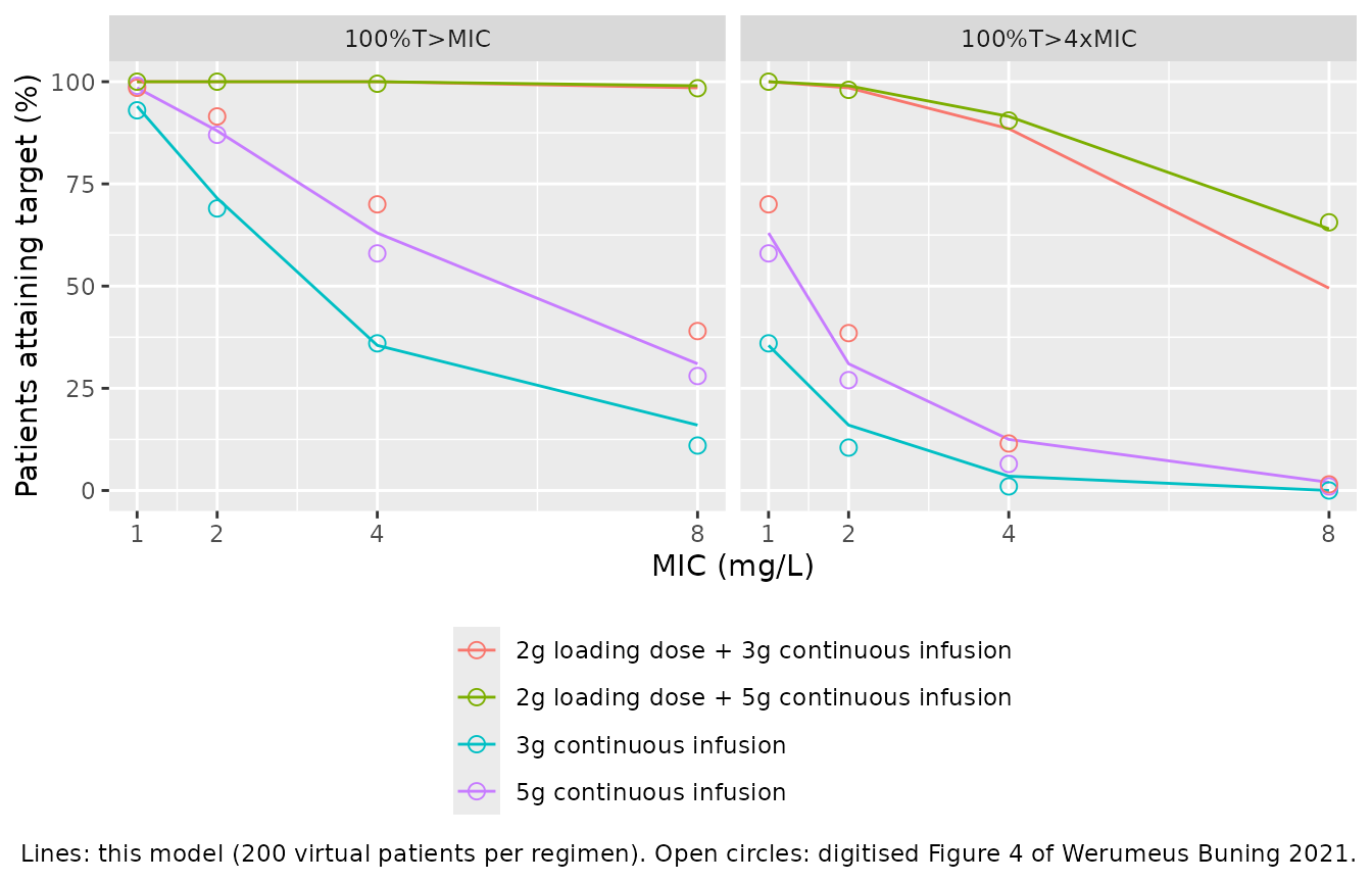
cmp |>
  select(regimen, target, mic, pta_pub, pta, diff) |>
  mutate(pta = round(pta, 1), diff = round(diff, 1)) |>
  dplyr::rename(
    "Regimen" = regimen, "Target" = target, "MIC (mg/L)" = mic,
    "Published (%)" = pta_pub, "Simulated (%)" = pta,
    "Difference (points)" = diff
  ) |>
knitr::kable(caption = "Probability of target attainment in the first 24 h: Figure 4 versus this model.")| Regimen | Target | MIC (mg/L) | Published (%) | Simulated (%) | Difference (points) |
|---|---|---|---|---|---|
| 3g continuous infusion | 100%T>MIC | 1 | 93.0 | 94.0 | 1.0 |
| 3g continuous infusion | 100%T>MIC | 2 | 69.0 | 71.5 | 2.5 |
| 3g continuous infusion | 100%T>MIC | 4 | 36.0 | 35.5 | -0.5 |
| 3g continuous infusion | 100%T>MIC | 8 | 11.0 | 16.0 | 5.0 |
| 5g continuous infusion | 100%T>MIC | 1 | 99.0 | 98.5 | -0.5 |
| 5g continuous infusion | 100%T>MIC | 2 | 87.0 | 88.0 | 1.0 |
| 5g continuous infusion | 100%T>MIC | 4 | 58.0 | 63.0 | 5.0 |
| 5g continuous infusion | 100%T>MIC | 8 | 28.0 | 31.0 | 3.0 |
| 2g loading dose + 3g continuous infusion | 100%T>MIC | 1 | 98.5 | 100.0 | 1.5 |
| 2g loading dose + 3g continuous infusion | 100%T>MIC | 2 | 91.5 | 100.0 | 8.5 |
| 2g loading dose + 3g continuous infusion | 100%T>MIC | 4 | 70.0 | 100.0 | 30.0 |
| 2g loading dose + 3g continuous infusion | 100%T>MIC | 8 | 39.0 | 98.5 | 59.5 |
| 2g loading dose + 5g continuous infusion | 100%T>MIC | 1 | 100.0 | 100.0 | 0.0 |
| 2g loading dose + 5g continuous infusion | 100%T>MIC | 2 | 100.0 | 100.0 | 0.0 |
| 2g loading dose + 5g continuous infusion | 100%T>MIC | 4 | 99.5 | 100.0 | 0.5 |
| 2g loading dose + 5g continuous infusion | 100%T>MIC | 8 | 98.4 | 99.0 | 0.6 |
| 3g continuous infusion | 100%T>4xMIC | 1 | 36.0 | 35.5 | -0.5 |
| 3g continuous infusion | 100%T>4xMIC | 2 | 10.5 | 16.0 | 5.5 |
| 3g continuous infusion | 100%T>4xMIC | 4 | 1.0 | 3.5 | 2.5 |
| 3g continuous infusion | 100%T>4xMIC | 8 | 0.0 | 0.0 | 0.0 |
| 5g continuous infusion | 100%T>4xMIC | 1 | 58.0 | 63.0 | 5.0 |
| 5g continuous infusion | 100%T>4xMIC | 2 | 27.0 | 31.0 | 4.0 |
| 5g continuous infusion | 100%T>4xMIC | 4 | 6.5 | 12.5 | 6.0 |
| 5g continuous infusion | 100%T>4xMIC | 8 | 1.0 | 2.0 | 1.0 |
| 2g loading dose + 3g continuous infusion | 100%T>4xMIC | 1 | 70.0 | 100.0 | 30.0 |
| 2g loading dose + 3g continuous infusion | 100%T>4xMIC | 2 | 38.5 | 98.5 | 60.0 |
| 2g loading dose + 3g continuous infusion | 100%T>4xMIC | 4 | 11.5 | 88.5 | 77.0 |
| 2g loading dose + 3g continuous infusion | 100%T>4xMIC | 8 | 1.5 | 49.5 | 48.0 |
| 2g loading dose + 5g continuous infusion | 100%T>4xMIC | 1 | 100.0 | 100.0 | 0.0 |
| 2g loading dose + 5g continuous infusion | 100%T>4xMIC | 2 | 98.0 | 99.0 | 1.0 |
| 2g loading dose + 5g continuous infusion | 100%T>4xMIC | 4 | 90.5 | 91.5 | 1.0 |
| 2g loading dose + 5g continuous infusion | 100%T>4xMIC | 8 | 65.6 | 64.0 | -1.6 |
Three of the four regimens reproduce Figure 4 across all MICs and both targets. The fourth does not: the curve labelled “2 g loading dose + 3 g continuous infusion” lies far below what the model gives for that regimen (at MIC 8 the paper shows 39% for 100% T > MIC; the model gives nearly 100%, because a 2 g bolus into a 46.8 L volume starts the typical patient at 43 mg/L). The same curve is instead reproduced, within about 5 points at every plotted MIC and for both targets, by 6 g per 24 h given by continuous infusion without a loading dose (table below). The concentrations of the paper’s own simulation are not available, so the reason cannot be settled. One possibility that fits is that the loading dose was entered as an infusion at the maintenance rate rather than as a bolus, which doubles the infusion rate over the first hours without the immediate jump in concentration. The companion 2 g + 5 g regimen, which the Results text and Conclusions recommend, does reproduce as a bolus.
matched <- cmp |>
  filter(regimen != "2g loading dose + 3g continuous infusion")
ld3_as_6g <- published |>
  filter(regimen == "2g loading dose + 3g continuous infusion") |>
  left_join(
    pta |>
      filter(regimen == "6g continuous infusion (no loading dose)") |>
      select(-regimen),
    by = c("target", "mic")
  )
ld3_as_labelled <- cmp |>
  filter(regimen == "2g loading dose + 3g continuous infusion")
stopifnot(
  nrow(matched) == 24L, nrow(ld3_as_6g) == 8L, !anyNA(ld3_as_6g$pta),
  # The etas are drawn with base R, so these statistics are identical on every
  # machine. 200 patients carry a binomial SE of up to 3.5 points and the
  # paper's 1000 up to 1.6; a mis-transcribed CL, V, exponent or IIV moves
  # the mid-range points by 10-30 points.
  median(abs(matched$diff)) < 4,
  max(abs(matched$diff)) < 10,
  median(abs(ld3_as_6g$pta - ld3_as_6g$pta_pub)) < 4,
  max(abs(ld3_as_6g$pta - ld3_as_6g$pta_pub)) < 10,
  # The deviation recorded above is real: as labelled, the regimen is far
  # above the published curve at MIC 8.
  ld3_as_labelled$diff[ld3_as_labelled$target == "100%T>MIC" &
    ld3_as_labelled$mic == 8] > 40
)

ld3_as_6g |>
  mutate(pta = round(pta, 1), diff = round(pta - pta_pub, 1)) |>
  select(target, mic, pta_pub, pta, diff) |>
  dplyr::rename(
    "Target" = target, "MIC (mg/L)" = mic,
    "Figure 4, '2 g LD + 3 g CI' (%)" = pta_pub,
    "Model, 6 g/24 h CI, no LD (%)" = pta,
    "Difference (points)" = diff
  ) |>
knitr::kable(caption = "The Figure 4 '2 g loading dose + 3 g' curve against a 6 g/24 h infusion without loading dose.")| Target | MIC (mg/L) | Figure 4, ‘2 g LD + 3 g CI’ (%) | Model, 6 g/24 h CI, no LD (%) | Difference (points) |
|---|---|---|---|---|
| 100%T>MIC | 1 | 98.5 | 99.0 | 0.5 |
| 100%T>MIC | 2 | 91.5 | 94.0 | 2.5 |
| 100%T>MIC | 4 | 70.0 | 71.5 | 1.5 |
| 100%T>MIC | 8 | 39.0 | 35.5 | -3.5 |
| 100%T>4xMIC | 1 | 70.0 | 71.5 | 1.5 |
| 100%T>4xMIC | 2 | 38.5 | 35.5 | -3.0 |
| 100%T>4xMIC | 4 | 11.5 | 16.0 | 4.5 |
| 100%T>4xMIC | 8 | 1.5 | 3.5 | 2.0 |
Replicate Figure 3: median concentration-time profiles
Figure 3 shows the median of 1000 virtual patients over the first 24 h for the 3 g continuous infusion and for the 2 g loading dose + 5 g regimen, first at the 10th, 50th and 90th percentiles of eGFR (33, 73 and 122 mL/min/1.73 m^2, comorbidity ‘other’), then for each comorbidity at the median eGFR.
fig3_scen <- tibble::tribble(
  ~panel, ~group, ~crcl, ~heme, ~trauma,
  "eGFR", "eGFR 33", 33, 0L, 0L,
  "eGFR", "eGFR 73", 73, 0L, 0L,
  "eGFR", "eGFR 122", 122, 0L, 0L,
  "Comorbidity", "other", 73, 0L, 0L,
  "Comorbidity", "hematologic malignancy", 73, 1L, 0L,
  "Comorbidity", "trauma or head injury", 73, 0L, 1L
)
fig3_reg <- regimens |> filter(regimen %in% c(
  "3g continuous infusion", "2g loading dose + 5g continuous infusion"
))

fig3 <- tidyr::crossing(fig3_scen, fig3_reg) |>
  rowwise() |>
  mutate(sim = list(simulate_regimen(
    ld_mg, daily_mg,
    covs = typical_covs(n_sub, crcl = crcl, heme = heme, trauma = trauma)
  ))) |>
  ungroup() |>
  select(panel, group, regimen, sim) |>
  tidyr::unnest(sim) |>
  group_by(panel, group, regimen, time) |>
  summarise(median = median(Cc), .groups = "drop")
#> ℹ omega/sigma items treated as zero: 'etalcl', 'etalvc'
#> ℹ omega/sigma items treated as zero: 'etalcl', 'etalvc'
#> ℹ omega/sigma items treated as zero: 'etalcl', 'etalvc'
#> ℹ omega/sigma items treated as zero: 'etalcl', 'etalvc'
#> ℹ omega/sigma items treated as zero: 'etalcl', 'etalvc'
#> ℹ omega/sigma items treated as zero: 'etalcl', 'etalvc'
#> ℹ omega/sigma items treated as zero: 'etalcl', 'etalvc'
#> ℹ omega/sigma items treated as zero: 'etalcl', 'etalvc'
#> ℹ omega/sigma items treated as zero: 'etalcl', 'etalvc'
#> ℹ omega/sigma items treated as zero: 'etalcl', 'etalvc'
#> ℹ omega/sigma items treated as zero: 'etalcl', 'etalvc'
#> ℹ omega/sigma items treated as zero: 'etalcl', 'etalvc'

ggplot(fig3, aes(time, median, colour = group)) +
  geom_line() +
  geom_hline(yintercept = c(8, 32), linetype = "dotted") +
  facet_grid(regimen ~ panel, scales = "free_y") +
  labs(
    x = "Time after first dose (h)", y = "Median ceftazidime (mg/L)",
    colour = NULL,
    caption = paste(
      "Replicates Figure 3 of Werumeus Buning 2021.",
      "Dotted lines: MIC 8 mg/L and 4 x MIC."
    )
  )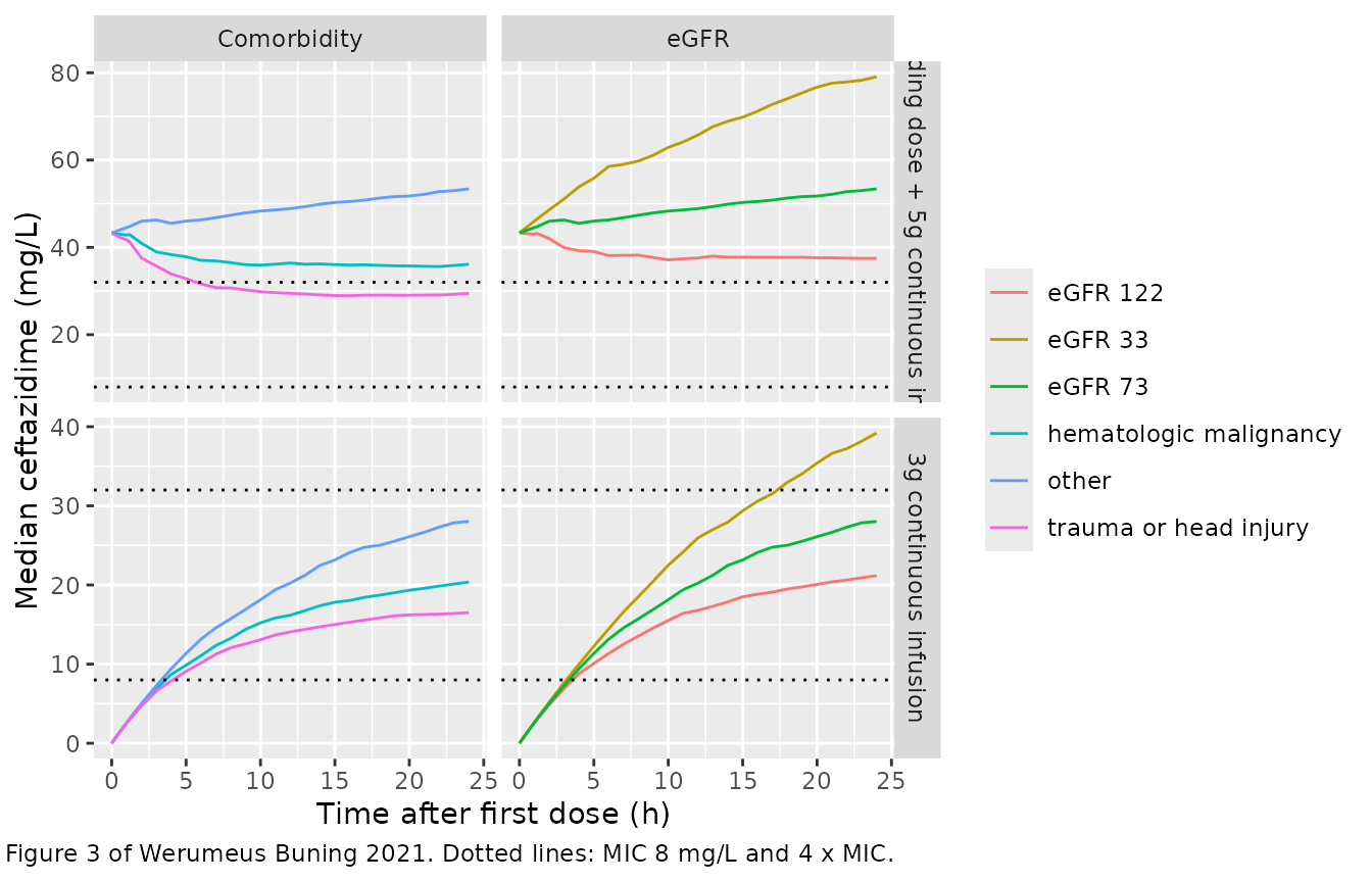
# 24-h medians read off Figure 3 by the maintainers (about +/- 1.5 mg/L).
fig3_pub <- tibble::tribble(
  ~regimen, ~group, ~pub,
  "3g continuous infusion", "eGFR 33", 38,
  "3g continuous infusion", "eGFR 73", 26.5,
  "3g continuous infusion", "eGFR 122", 20,
  "3g continuous infusion", "hematologic malignancy", 19,
  "3g continuous infusion", "trauma or head injury", 17,
  "2g loading dose + 5g continuous infusion", "eGFR 33", 77,
  "2g loading dose + 5g continuous infusion", "eGFR 73", 50,
  "2g loading dose + 5g continuous infusion", "eGFR 122", 35,
  "2g loading dose + 5g continuous infusion", "hematologic malignancy", 35,
  "2g loading dose + 5g continuous infusion", "trauma or head injury", 32
)
fig3_cmp <- fig3_pub |>
  left_join(
    fig3 |> filter(time == 24) |> select(regimen, group, median),
    by = c("regimen", "group")
  ) |>
  mutate(pct_diff = 100 * (median / pub - 1))
stopifnot(nrow(fig3_cmp) == 10L, !anyNA(fig3_cmp$median))

fig3_cmp |>
  mutate(median = round(median, 1), pct_diff = round(pct_diff, 1)) |>
  dplyr::rename(
    "Regimen" = regimen, "Group" = group, "Figure 3 (mg/L)" = pub,
    "Simulated median (mg/L)" = median, "Difference (%)" = pct_diff
  ) |>
knitr::kable(caption = "Median concentration at 24 h: Figure 3 versus this model.")| Regimen | Group | Figure 3 (mg/L) | Simulated median (mg/L) | Difference (%) |
|---|---|---|---|---|
| 3g continuous infusion | eGFR 33 | 38.0 | 39.2 | 3.2 |
| 3g continuous infusion | eGFR 73 | 26.5 | 28.0 | 5.8 |
| 3g continuous infusion | eGFR 122 | 20.0 | 21.2 | 5.9 |
| 3g continuous infusion | hematologic malignancy | 19.0 | 20.4 | 7.2 |
| 3g continuous infusion | trauma or head injury | 17.0 | 16.5 | -2.9 |
| 2g loading dose + 5g continuous infusion | eGFR 33 | 77.0 | 79.1 | 2.7 |
| 2g loading dose + 5g continuous infusion | eGFR 73 | 50.0 | 53.4 | 6.8 |
| 2g loading dose + 5g continuous infusion | eGFR 122 | 35.0 | 37.5 | 7.1 |
| 2g loading dose + 5g continuous infusion | hematologic malignancy | 35.0 | 36.1 | 3.2 |
| 2g loading dose + 5g continuous infusion | trauma or head injury | 32.0 | 29.4 | -8.0 |
stopifnot(
  # Centre and envelope, not extremes. A mis-transcribed exponent or
  # comorbidity factor moves the affected rows by 25-100%.
  abs(median(fig3_cmp$pct_diff)) < 8,
  quantile(abs(fig3_cmp$pct_diff), 0.9) < 15
)
The eGFR and comorbidity effects reproduce Figure 3. The model’s median at 24 h in trauma or head injury patients on the 2 g + 5 g regimen sits about 8% below the published curve, and the other rows sit 3-7% above it; both are within what can be read from the figure.
PKNCA: steady-state mass balance
The paper reports no non-compartmental results. As a check that the dose, volume and clearance units are consistent, a typical patient receiving 5 g per 24 h by continuous infusion for 10 days (more than 25 half-lives) must have an AUC over the last day equal to the daily dose divided by clearance, in each eGFR and comorbidity stratum.
ss_scen <- scen |>
  filter(cvvh == 0L) |>
  mutate(treatment = label)
ev_ss <- ss_scen |>
  transmute(
    id, treatment, CRCL = crcl, DIS_HEME_MALIG = heme,
    DIS_TRAUMA = trauma, RRT_CRRT_STATUS = cvvh
  )
ev_ss <- bind_rows(
  ev_ss |> mutate(
    time = 0, amt = 50000, rate = 5000 / 24, evid = 1L, cmt = "central"
  ),
  ev_ss |>
    tidyr::crossing(time = c(0, seq(216, 240, by = 0.5))) |>
    mutate(amt = 0, rate = 0, evid = 0L, cmt = "central")
) |>
  arrange(id, time, desc(evid))

sim_ss <- rxode2::rxSolve(
  mod_typ, events = ev_ss, keep = c("treatment"),
  rtol = 1e-10, atol = 1e-12
) |>
  as.data.frame()
#> ℹ omega/sigma items treated as zero: 'etalcl', 'etalvc'
#> Warning: multi-subject simulation without without 'omega'

conc_obj <- PKNCA::PKNCAconc(
  sim_ss |> filter(!is.na(Cc)) |> select(id, treatment, time, Cc),
  Cc ~ time | treatment + id
)
dose_obj <- PKNCA::PKNCAdose(
  ev_ss |> filter(evid == 1L) |> select(id, treatment, time, amt),
  amt ~ time | treatment + id
)
intervals <- data.frame(start = 216, end = 240, auclast = TRUE)
nca <- PKNCA::pk.nca(PKNCA::PKNCAdata(conc_obj, dose_obj, intervals = intervals))

ss_cmp <- as.data.frame(nca) |>
  filter(PPTESTCD == "auclast") |>
  left_join(
    sim_ss |> group_by(treatment) |> summarise(cl = first(cl)),
    by = "treatment"
  ) |>
  mutate(ratio = PPORRES * cl / 5000)
stopifnot(nrow(ss_cmp) == 5L, max(abs(ss_cmp$ratio - 1)) < 1e-3)

ss_cmp |>
  transmute(
    Stratum = treatment,
    "AUC 216-240 h (mg*h/L)" = signif(PPORRES, 5),
    "CL (L/h)" = signif(cl, 4),
    "AUC x CL / daily dose" = signif(ratio, 5)
  ) |>
knitr::kable(caption = "Steady-state AUC over one day times clearance equals the daily dose.")| Stratum | AUC 216-240 h (mg*h/L) | CL (L/h) | AUC x CL / daily dose |
|---|---|---|---|
| hematologic malignancy | 931.20 | 5.369 | 1.00000 |
| other, eGFR 122 | 983.47 | 5.084 | 1.00000 |
| other, eGFR 33 | 2698.30 | 1.853 | 0.99988 |
| other, eGFR 73 | 1462.00 | 3.420 | 1.00000 |
| trauma or head injury | 734.67 | 6.806 | 1.00000 |
Assumptions and deviations
- The “2 g loading dose + 3 g continuous infusion” curve of Figure 4 is not reproduced as labelled. It matches 6 g per 24 h by continuous infusion without a loading dose at all eight plotted points (within about 5 percentage points); the other three regimens reproduce. The model is shipped exactly as the Appendix C control stream prints it; see the Figure 4 section for the comparison.
-
Residual error. Table 2 calls the residual error
“proportional”, but the control stream fits log-transformed
concentrations with
Y = LOG(F) + THETA(1)*EPS(1)and$SIGMA 1 FIX. That is an additive error of SD 0.281 on the log scale, encoded aslnorm(expSd). - eGFR units. Table 1 prints the eGFR unit as mL/min/m^2. The CKD-EPI 2009 equation named in Section 4.4 is normalised to 1.73 m^2, and the covariate is used as mL/min/1.73 m^2 here. Because it enters as a ratio to the median of 73, the reading does not change the model as long as values come from the same equation.
- CVVH patients. On CVVH, clearance is a fixed 2.9 L/h with no between-subject variability and no eGFR or comorbidity effect, as in the control stream. The eGFR column must still hold a finite value for these patients (any value; it is multiplied by zero).
-
Comorbidity coding. The source recorded one
comorbidity category per patient, so
DIS_HEME_MALIGandDIS_TRAUMAwere never both 1 in the fitted data. The reference group (‘other’) includes the oncologic (solid) malignancy category, which had no retained effect. Head injury without other trauma counts asDIS_TRAUMA = 1because the authors merged the two categories. - Below-quantification data were handled with the M5 method (7.1% of samples); this affects estimation only and has no counterpart in the model file.
- Target-attainment simulations use the individual predictions without residual error, 200 virtual patients per regimen rather than the paper’s 1000, and the typical covariates the paper states for Figure 4 (median eGFR 73, comorbidity ‘other’). The paper does not say whether its simulated patients were on CVVH; they are taken as not on CVVH, since the figure caption fixes the eGFR, which only acts off CVVH.
- Protein binding. The paper measured total concentrations and states that ceftazidime is about 10% bound; the targets are applied to total concentration, as in the paper.