CD123 NK cell engager translational PK/PD (Choi 2024)
Source:vignettes/articles/Choi_2024_cd123nkce.Rmd
Choi_2024_cd123nkce.RmdModel and source
Choi et al. (2024) built a translational, synapse-driven PK/PD model for CD123-NKCE, a trifunctional natural killer cell engager that binds NKp46 and CD16a on NK cells and CD123 on acute myeloid leukemia (AML) cells. The translation runs in three steps, and each is a separate model here:
-
Choi_2024_cd123nkce_invitro: MOLM-13 cytotoxicity in vitro, which estimates the synapse parameterskmax,EC50andgamma. -
Choi_2024_cd123nkce_nhp: PK, CD123+ cells and NKp46+ NK cells in healthy monkeys, with the synapse parameters carried over from step 1. -
Choi_2024_cd123nkce_human: the projection to patients with AML that was used to select the first-in-human starting regimen.
- Citation: Choi SL, Valente D, Virone-Oddos A, Mauriac C. Developing a mechanistic translational PK/PD model for a trifunctional NK cell engager to predict the first-in-human dose for acute myeloid leukemia. Clin Transl Sci. 2024;17(1):e13689. doi:10.1111/cts.13689
- Article: https://doi.org/10.1111/cts.13689 (open access; the model equations and the Monolix script for the AML model are in Appendix S1)
All three models share one structure. CD123-NKCE binds NKp46 on NK
cells (drug_nkp46_central) and CD123 on CD123+ cells
(drug_cd123_central); either binary complex then binds the
other receptor to form the NKp46-drug-CD123 synapse
(trimer). The synapse kills CD123+ cells at the Hill rate
kmax * TBE^gamma / (EC50^gamma + TBE^gamma). Binding to
CD16a is ignored because its affinity is about 150-fold weaker than for
NKp46. The in vivo models add two-compartment PK, internalisation of
drug-CD123 complexes, an extra turned-over CD123 pool outside the blood
(target / complex, the main target-mediated
drug sink), and synapse-driven redistribution of NK cells out of the
blood.
Population
- In vitro: resting NK cells from two donors against 51Cr-labelled MOLM-13 cells at effector-to-target (E:T) ratios of 10:1, 5:1, 1:1 and 1:5 (20 MOLM-13 cells/uL), eight drug concentrations from 1.5e-3 to 1.5e4 ng/mL, and incubations of 1, 4 and 20 h.
- Monkeys: 53 healthy animals in five studies (Table S1): IV 1-h infusions of 0.5-3000 ug/kg (single dose, weekly or twice weekly) and SC doses of 3.6-3000 ug/kg. Twenty-three animals contributed PK and PD to the fit; the 30 animals dosed twice weekly contributed PK only, and their PD data served as external validation.
- AML patients: a projection with no clinical data. Baseline NKp46+ NK cells were 54 cells/uL and CD123+ cells 1668 cells/uL (Table 1).
str(readModelDb("Choi_2024_cd123nkce_nhp")()$population)
#> List of 7
#>  $ species       : chr "nonhuman primate (monkey)"
#>  $ n_subjects    : num 53
#>  $ n_studies     : num 5
#>  $ sex_female_pct: num 41.5
#>  $ disease_state : chr "Healthy"
#>  $ dose_range    : chr "IV 1-h infusion 0.5-3000 ug/kg (single, weekly or twice weekly); SC 3.6-3000 ug/kg (single or twice weekly)"
#>  $ notes         : chr "Five studies (Table S1): study 1, 3000 ug/kg IV single dose (3 females); study 2, 0.5, 3 and 3000 ug/kg IV and "| __truncated__
Source trace
Every ini() value carries an in-file comment that points
to its source. The table below collects them. “Table 1” is the main-text
parameter table; “Eq” numbers refer to Appendix S1, and “Table S2” is
the Monolix script of the AML model.
| Parameter (model name) | In vitro | Monkey | AML | Source |
|---|---|---|---|---|
kmax (1/h) |
0.332 (est.) | 0.332 (fixed) | 0.332 (fixed) | Table 1 |
EC50 (nM) |
1.46e-9 (est., IIV SD 0.998) | 1.46e-9 | 1.46e-9 | Table 1 |
gamma (hill) |
1.04 (est.) | 1.04 | 1.04 | Table 1 |
kg (1/h) |
0.0139 | 0.31 (IIV SD 0.83) | 0.0288 | Table 1 |
kout NK (1/h) |
– | 0.2 | 0.002 | Table 1 |
KD1 NKp46 (nM) |
16.6 | 29 | 16.6 | Table 1 |
KD2 CD123 (nM) |
0.404 | 1.23 | 0.404 | Table 1 |
koff1, koff2 (1/s) |
0.001 | 0.001 | 0.001 | Table 1 |
RTdE (nkp46_receptors) |
4600 | 4600 | 4600 | Table 1 |
RTdT (cd123_receptors) |
4360 | 25,000 | 7000 | Table 1 |
EF0 (rbase_nk, cells/uL) |
4-200 (per well) | median 247 | 54 | Table 1 |
TC0 (rbase_cd123, cells/uL) |
20 | median 28 | 1668 | Table 1 |
CL (mL/h/kg) |
– | 0.32 (IIV SD 0.20) | 0.18 | Table 1 |
Q (mL/h/kg) |
– | 1.35 | 0.37 | Table 1 |
V1 (L/kg) |
– | 0.040 (IIV SD 0.130) | 0.042 | Table 1 |
V2 (L/kg) |
– | 0.020 (IIV SD 0.26) | 0.031 | Table 1 |
ka (1/h) |
– | 0.04 | – | Table 1 |
F |
– | 74.0% (logit IIV SD 0.28) | – | Table 1 |
kint (1/h) |
– | 0.15 | 0.15 | Table 1 |
kinTP (ksyn, nM/h) |
– | 0.21 (IIV SD 0.57) | 0.21 | Table 1 |
alpha (target_scale, nM) |
– | 19.44 (IIV SD 0.61) | 19.44 | Table 1 |
beta (target_exp) |
– | 0.21 | 0.21 | Table 1 |
SlpNK (slope_nk) |
– | 5.72 | 5.72 | Table 1 |
TADA (h) |
– | 333 (IIV SD 0.20) | – | Table 1 |
KADA (1/h) |
– | 1.94 (IIV SD 4.21) | – | Table 1 |
ktol (1/h) |
– | 0.0032 (IIV SD 1.63) | – | Table 1 |
delta (delta_tol) |
– | 0.18 (IIV SD 0.53) | – | Table 1 |
TCmax (cells/uL) |
– | – | 3252 | Table 1 |
| Molecular weight (g/mol) | – | 149,000 | 149,000 | Table S2 |
| Avogadro’s number | 6.022e14 /nmol | same | same | Table S2 |
| Binding ODEs | Eqs 1-4 | Eqs 2, 4, 14-17 | Table S2 | Appendix S1 |
| Killing rate | Eq 8 | Eq 8 | Table S2 kel
|
Appendix S1 |
Free receptors E, T
|
Eqs 9-10 | Table S2 | Table S2 | Appendix S1 |
Non-blood CD123 baseline TP0
|
– | Eq 18 | Table S2 | Appendix S1 |
| NK redistribution | – | Eq 19 | Table S2 ddt_EF
|
Appendix S1 |
| CD123+ growth | Eqs 6-7 | Eqs 20-21 (tolerance) | Table S2 ddt_TA (logistic) |
Appendix S1 |
| ADA switch | – | Eq 14 | – | Appendix S1 |
The IIV column of Table 1 reports the standard deviation of each
random effect, so the ini() variances are its squares. All
random effects are log-normal except F, which is
logit-normal (Table 1 footnote p).
In vitro cytotoxicity (Figure 3)
The in vitro model is deterministic apart from the inter-experiment
variability on EC50, which is zeroed here to reproduce the
typical curves of Figure 3. The drug concentration enters as an
amt in nM at time 0. Figure 3 plots the concentration in
ng/mL, and Table 1 gives the same range as 1.02e-5 to 102 nM, so ng/mL
is converted with that ratio (102 / 1.5e4, i.e. a molecular weight of
about 147 kDa).
mod_iv <- readModelDb("Choi_2024_cd123nkce_invitro") |> rxode2::zeroRe()
#> ℹ parameter labels from comments will be replaced by 'label()'
#> Warning: No sigma parameters in the model

conc_ngml <- 1.5 * 10^(-3:4)
et_design <- tibble::tibble(
  et_label = factor(c("10:1", "5:1", "1:1", "1:5"), levels = c("10:1", "5:1", "1:1", "1:5")),
  rbase_nk = c(200, 100, 20, 4)
)
wells <- tidyr::expand_grid(et_design, conc_ngml = conc_ngml) |>
  mutate(id = dplyr::row_number())

iv_events <- dplyr::bind_rows(
  wells |> mutate(time = 0, amt = conc_ngml * 102 / 1.5e4, evid = 1L, cmt = "central"),
  tidyr::expand_grid(wells, time = c(1, 4, 20)) |>
    mutate(amt = 0, evid = 0L, cmt = "central")
) |>
  arrange(id, time, dplyr::desc(evid))

sim_iv <- rxode2::rxSolve(
  mod_iv,
  events = iv_events,
  keep = c("et_label", "conc_ngml"),
  returnType = "data.frame"
)
#> ℹ omega/sigma items treated as zero: 'etalec50'
sim_iv |>
  ggplot(aes(conc_ngml, cytotox, colour = et_label)) +
  geom_line() +
  geom_point(size = 1) +
  facet_grid(et_label ~ paste(time, "h")) +
  scale_x_log10() +
  coord_cartesian(ylim = c(0, 100)) +
  labs(
    x = "CD123-NKCE (ng/mL)", y = "Cytotoxicity (%)", colour = "E:T",
    caption = "Replicates the typical model curves of Figure 3 of Choi 2024."
  )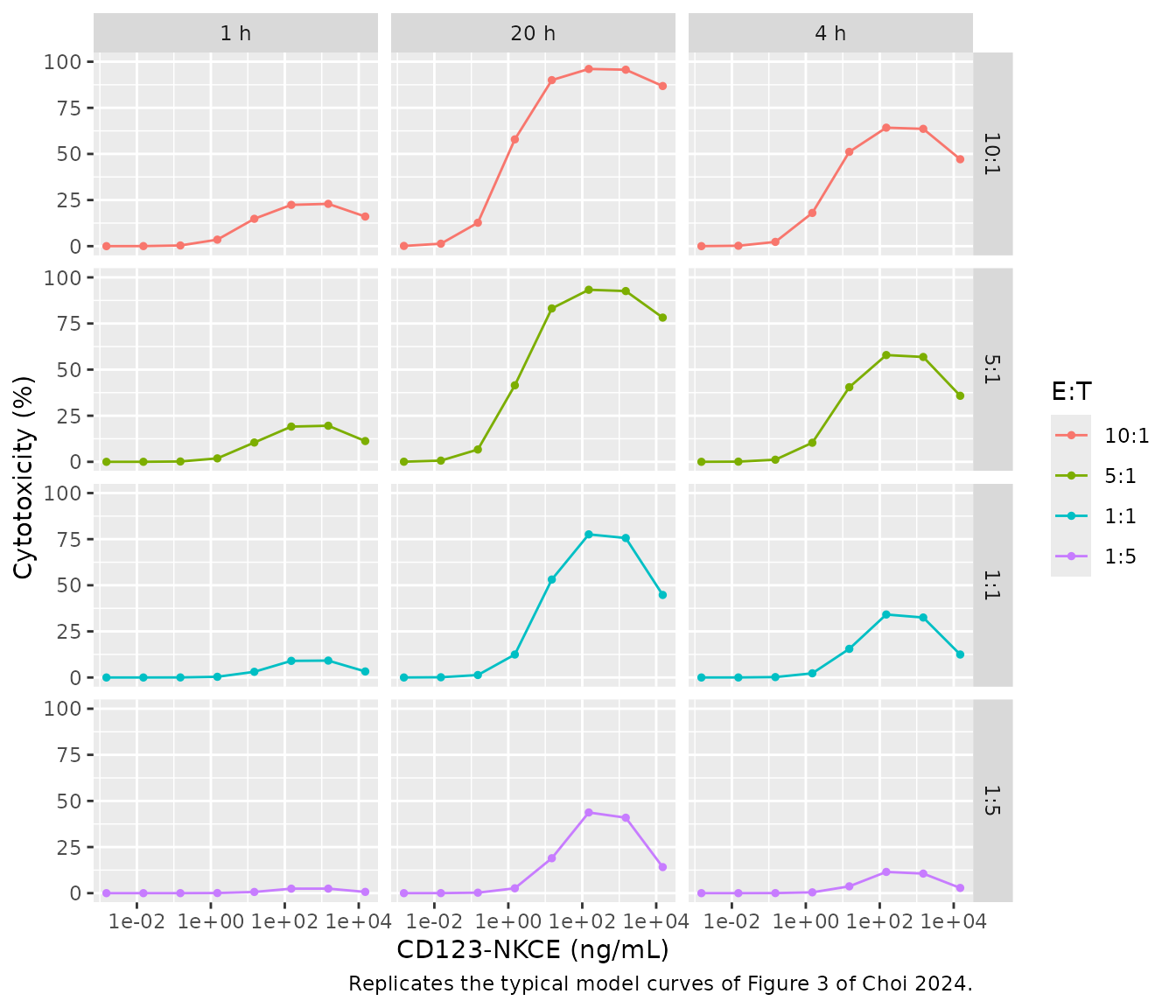
The curves reproduce Figure 3: killing rises with E:T ratio and incubation time, and every panel is bell-shaped, because at the highest concentrations both receptors are saturated by binary complexes and fewer synapses form.
The free-CD123 term
Appendix S1 Eq 10 writes the total CD123 pool from the
baseline target-cell count TC0, and the text says
that “the number of cells remains constant in vitro”. The Monolix script
of the AML model (Table S2) instead uses the current target-cell count
(TC = TA * RTdT). The packaged model uses the current,
surviving-cell count. The comparison below shows why: with the published
estimates, only that form reproduces the typical curves of Figure 3. The
reference values were read by the maintainers from Figure 3 and are
accurate to a few percentage points.
fig3 <- tibble::tribble(
  ~et_label, ~time, ~conc_ngml, ~fig3,
  "10:1", 1, 150, 22,
  "10:1", 4, 150, 62,
  "10:1", 20, 15000, 85,
  "5:1", 20, 150, 95,
  "5:1", 20, 15000, 78,
  "1:1", 4, 150, 33,
  "1:1", 20, 150, 77,
  "1:1", 20, 15000, 45,
  "1:5", 20, 150, 43,
  "1:5", 20, 15000, 15
)

# The printed Eq 10: total CD123 fixed at the baseline cell count.
mod_iv_eq10 <- readModelDb("Choi_2024_cd123nkce_invitro") |>
  rxode2::model(
    tfree <- rbase_cd123 * cd123_receptors * 1e6 / navo - drug_cd123_central - trimer
  ) |>
  rxode2::zeroRe()
#> ℹ parameter labels from comments will be replaced by 'label()'
#> Warning: No sigma parameters in the model
sim_iv_eq10 <- rxode2::rxSolve(
  mod_iv_eq10,
  events = iv_events,
  keep = c("et_label", "conc_ngml"),
  returnType = "data.frame"
)
#> ℹ omega/sigma items treated as zero: 'etalec50'

lookup <- function(sim, et, tm, cc) {
  v <- sim$cytotox[as.character(sim$et_label) == et & sim$time == tm & abs(sim$conc_ngml - cc) < 1e-6 * cc]
  if (length(v) != 1L) stop("no unique row for ", et, " / ", tm, " h / ", cc, " ng/mL")
  v
}
fig3_check <- fig3 |>
  rowwise() |>
  mutate(
    packaged = lookup(sim_iv, et_label, time, conc_ngml),
    printed_eq10 = lookup(sim_iv_eq10, et_label, time, conc_ngml)
  ) |>
  ungroup()

fig3_check |>
  mutate(across(c(packaged, printed_eq10), \(x) round(x, 1))) |>
  dplyr::rename(
    "E:T" = et_label, "Time (h)" = time, "Concentration (ng/mL)" = conc_ngml,
    "Figure 3 (%)" = fig3, "Packaged model (%)" = packaged,
    "Printed Eq 10 (%)" = printed_eq10
  ) |>
knitr::kable()| E:T | Time (h) | Concentration (ng/mL) | Figure 3 (%) | Packaged model (%) | Printed Eq 10 (%) |
|---|---|---|---|---|---|
| 10:1 | 1 | 150 | 22 | 22.4 | 22.7 |
| 10:1 | 4 | 150 | 62 | 64.2 | 67.5 |
| 10:1 | 20 | 15000 | 85 | 86.8 | 97.6 |
| 5:1 | 20 | 150 | 95 | 93.3 | 99.3 |
| 5:1 | 20 | 15000 | 78 | 78.2 | 92.2 |
| 1:1 | 4 | 150 | 33 | 34.2 | 37.6 |
| 1:1 | 20 | 150 | 77 | 77.6 | 91.6 |
| 1:1 | 20 | 15000 | 45 | 44.8 | 50.1 |
| 1:5 | 20 | 150 | 43 | 43.8 | 48.6 |
| 1:5 | 20 | 15000 | 15 | 14.1 | 13.3 |
Monkey PK/PD (Figure 4)
Deterministic checks
The paper states that, at the median baseline of 28 CD123+ cells/uL, the blood CD123 pool is 0.0011 nM and the non-blood pool is 4.70 nM (Discussion). Both follow from Eq 18 and the Table 1 values, and the typical model reproduces them as the steady state before dosing.
mod_nhp <- readModelDb("Choi_2024_cd123nkce_nhp")
mod_nhp_typ <- mod_nhp |> rxode2::zeroRe()
#> ℹ parameter labels from comments will be replaced by 'label()'
#> Warning: No sigma parameters in the model

sim_pre <- rxode2::rxSolve(
  mod_nhp_typ,
  events = rxode2::et(c(0, 24, 168)),
  returnType = "data.frame"
)
#> ℹ omega/sigma items treated as zero: 'etalcl', 'etalvc', 'etalvp', 'etalogitfdepot', 'etaltada', 'etalkada', 'etalksyn', 'etaltarget_scale', 'etalkg', 'etalktol', 'etaldelta_tol'
blood_cd123_0 <- 28 * 25000 * 1e6 / 6.022e14
c(blood_nM = blood_cd123_0, nonblood_nM = sim_pre$target[1])
#>    blood_nM nonblood_nM
#> 0.001162405 4.703501547
stopifnot(
  abs(blood_cd123_0 / 0.0011 - 1) < 0.06,
  abs(sim_pre$target[1] / 4.70 - 1) < 0.01,
  # No dose: the non-blood pool and the cell counts stay at baseline.
  max(abs(sim_pre$target / sim_pre$target[1] - 1)) < 1e-4,
  max(abs(sim_pre$cd123cell_central / 28 - 1)) < 1e-4
)
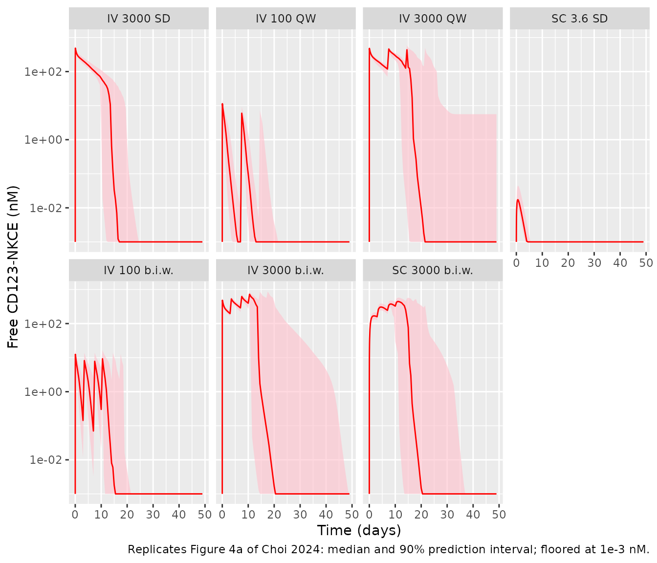
A 3000 ug/kg IV dose is 20.1 nmol/kg, which in the 0.040 L/kg central volume is 503 nM before any binding or elimination. The simulated end-of-infusion concentration sits just below that, as in Figure 4a (about 500 nM).
ev_3000 <- rxode2::et(amt = 3000, time = 0, cmt = "central", dur = 1) |>
  rxode2::et(c(0.5, 1, 2, 24))
sim_3000 <- rxode2::rxSolve(mod_nhp_typ, events = ev_3000, returnType = "data.frame")
#> ℹ omega/sigma items treated as zero: 'etalcl', 'etalvc', 'etalvp', 'etalogitfdepot', 'etaltada', 'etalkada', 'etalksyn', 'etaltarget_scale', 'etalkg', 'etalktol', 'etaldelta_tol'
c0 <- 3000 * 1e3 / 149000 / 0.040
cmax_typ <- sim_3000$Cc[sim_3000$time == 1]
c(closed_form_nM = c0, simulated_eoi_nM = cmax_typ)
#>   closed_form_nM simulated_eoi_nM
#>         503.3557         488.4655
stopifnot(cmax_typ < c0, cmax_typ / c0 > 0.9)
Visual predictive check
rxode2::rxSetSeed(20240103)
n_per_arm <- 50L

h <- function(days) days * 24
nhp_arms <- tibble::tribble(
  ~arm,                ~route,    ~dose,  ~dose_days,
  "IV 3000 SD",        "IV",      3000,   list(0),
  "IV 100 QW",         "IV",      100,    list(c(0, 7, 14, 21)),
  "IV 3000 QW",        "IV",      3000,   list(c(0, 7, 14, 21)),
  "SC 3.6 SD",         "SC",      3.6,    list(0),
  "IV 100 b.i.w.",     "IV",      100,    list(c(0, 3, 7, 10, 14, 17, 21, 24, 28)),
  "IV 3000 b.i.w.",    "IV",      3000,   list(c(0, 3, 7, 10, 14, 17, 21, 24, 28)),
  "SC 3000 b.i.w.",    "SC",      3000,   list(c(0, 3, 7, 10, 14, 17, 21, 24, 28))
) |>
  mutate(arm = factor(arm, levels = arm), arm_index = dplyr::row_number())

obs_times <- sort(unique(c(seq(0, 2, by = 0.25), seq(3, 48, by = 3), seq(48, h(49), by = 12))))

make_arm <- function(arm_row) {
  ids <- (arm_row$arm_index - 1L) * n_per_arm + seq_len(n_per_arm)
  doses <- tidyr::expand_grid(id = ids, time = h(unlist(arm_row$dose_days))) |>
    mutate(
      evid = 1L, amt = arm_row$dose,
      cmt = if (arm_row$route == "IV") "central" else "depot",
      dur = if (arm_row$route == "IV") 1 else 0
    )
  obs <- tidyr::expand_grid(id = ids, time = obs_times) |>
    mutate(evid = 0L, amt = 0, cmt = "central", dur = 0)
  dplyr::bind_rows(doses, obs) |>
    mutate(arm = arm_row$arm)
}
nhp_events <- lapply(split(nhp_arms, nhp_arms$arm), make_arm) |>
  dplyr::bind_rows() |>
  arrange(id, time, dplyr::desc(evid))
stopifnot(!anyDuplicated(nhp_events[nhp_events$evid == 1L, c("id", "time")]))

sim_nhp <- rxode2::rxSolve(
  mod_nhp,
  events = nhp_events,
  keep = c("arm"),
  returnType = "data.frame",
  cores = 1L
)
#> ℹ parameter labels from comments will be replaced by 'label()'
vpc <- function(sim, var) {
  sim |>
    group_by(arm, time) |>
    summarise(
      Q05 = quantile(.data[[var]], 0.05, na.rm = TRUE),
      Q50 = quantile(.data[[var]], 0.50, na.rm = TRUE),
      Q95 = quantile(.data[[var]], 0.95, na.rm = TRUE),
      .groups = "drop"
    )
}
vpc(sim_nhp, "Cc") |>
  mutate(across(c(Q05, Q50, Q95), \(x) pmax(x, 1e-3))) |>
  ggplot(aes(time / 24, Q50)) +
  geom_ribbon(aes(ymin = Q05, ymax = Q95), fill = "pink", alpha = 0.6) +
  geom_line(colour = "red") +
  facet_wrap(~arm, ncol = 4) +
  scale_y_log10() +
  labs(
    x = "Time (days)", y = "Free CD123-NKCE (nM)",
    caption = "Replicates Figure 4a of Choi 2024: median and 90% prediction interval; floored at 1e-3 nM."
  )
sd_qw_arms <- c("IV 3000 SD", "IV 100 QW", "IV 3000 QW", "SC 3.6 SD")
dplyr::bind_rows(
  vpc(sim_nhp, "cd123cell_central") |> mutate(panel = "CD123+ cells (cells/uL)"),
  vpc(sim_nhp, "nkcell_central") |> mutate(panel = "NKp46+ NK cells (cells/uL)")
) |>
  filter(arm %in% sd_qw_arms) |>
  ggplot(aes(time / 24, Q50)) +
  geom_ribbon(aes(ymin = Q05, ymax = Q95), fill = "pink", alpha = 0.6) +
  geom_line(colour = "red") +
  facet_grid(panel ~ arm, scales = "free_y") +
  labs(
    x = "Time (days)", y = NULL,
    caption = "Replicates Figures 4b and 4c of Choi 2024: median and 90% prediction interval."
  )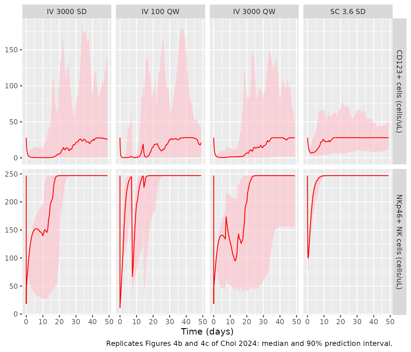
The simulations reproduce the main features of Figure 4. After 3000
ug/kg IV the concentration starts near 500 nM. It collapses around day
14, when anti-drug antibodies emerge (TADA = 333 h). From
then on the model adds the KADA elimination and stops
delivering further doses. That is why the third and fourth weekly doses
barely register in the median. CD123+ cells are depleted within a day
and recover once the drug is gone. NK cells fall during synapse
formation and return to baseline.
The CD123+ rebound in this model overshoots baseline and then
oscillates. That comes from the moderator-mediated tolerance term:
growth is driven by kg * (1 - (M/TC0)^delta), and the
moderator M lags the cell count with a 9-day half-life, so
the cells overshoot before M catches up. Individual fits in
Figure S1 show the same overshoot-and-return pattern. With the large IIV
on kg and ktol, the population median smooths
the oscillation.
The NK-cell prediction interval is narrower than in Figure 4c. The paper used each animal’s own baseline (144-1110 cells/uL) as a regressor, whereas these simulations hold every animal at the median baseline of 247 cells/uL.
med_at <- function(var, arm_name, t_h) {
  v <- sim_nhp[[var]][sim_nhp$arm == arm_name & sim_nhp$time == t_h]
  if (length(v) != n_per_arm) stop("expected ", n_per_arm, " rows for ", arm_name, " at ", t_h, " h")
  median(v)
}
stopifnot(
  # IV 3000 SD: median end-of-infusion concentration within 15% of 500 nM
  abs(med_at("Cc", "IV 3000 SD", 1) / 500 - 1) < 0.15,
  # CD123+ cells are depleted by more than 80% at 24 h in the median
  med_at("cd123cell_central", "IV 3000 SD", 24) < 0.2 * 28,
  # NK cells are back to within 10% of baseline 7 weeks after a single dose
  abs(med_at("nkcell_central", "IV 3000 SD", h(48)) / 247 - 1) < 0.1
)
Projection to patients with AML (Figure 5)
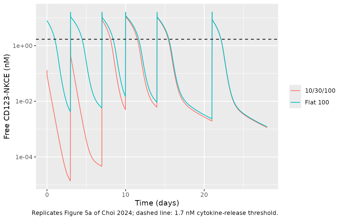
The paper looked for a starting regimen that met two criteria. First, the concentration at the end of the first infusion should stay below 1.7 nM, the lowest concentration that caused mild cytokine release in a whole-blood assay. Second, CD123+ cells should fall by more than 95% within the first 28-day cycle. Figure 5 compares a flat 100 ug/kg twice-weekly regimen with an intrapatient escalation of 10 and 30 ug/kg in week 1 followed by 100 ug/kg. Figure 5 draws doses on days 0, 3, 7, 10, 14 and 21, and that schedule is used here. The model has no variability, so these are typical-value solves. The Monolix script delivers each dose as a 0.0001-h input, which is equivalent to an IV bolus.
mod_aml <- readModelDb("Choi_2024_cd123nkce_human")
dose_days <- c(0, 3, 7, 10, 14, 21)
aml_regimens <- list(
  "Flat 100" = rep(100, 6),
  "10/30/100" = c(10, 30, 100, 100, 100, 100)
)
aml_obs <- sort(unique(c(seq(0, 2, by = 0.05), seq(0, h(28), by = 0.5))))
aml_events <- dplyr::bind_rows(lapply(seq_along(aml_regimens), function(i) {
  dplyr::bind_rows(
    tibble::tibble(id = i, time = h(dose_days), amt = aml_regimens[[i]], evid = 1L, cmt = "central"),
    tibble::tibble(id = i, time = aml_obs, amt = 0, evid = 0L, cmt = "central")
  ) |>
    mutate(regimen = names(aml_regimens)[i])
})) |>
  arrange(id, time, dplyr::desc(evid))

sim_aml <- rxode2::rxSolve(mod_aml, events = aml_events, keep = c("regimen"), returnType = "data.frame")
sim_aml |>
  filter(time > 0) |>
  ggplot(aes(time / 24, Cc, colour = regimen)) +
  geom_line() +
  geom_hline(yintercept = 1.7, linetype = "dashed") +
  scale_y_log10() +
  labs(
    x = "Time (days)", y = "Free CD123-NKCE (nM)", colour = NULL,
    caption = "Replicates Figure 5a of Choi 2024; dashed line: 1.7 nM cytokine-release threshold."
  )
sim_aml |>
  ggplot(aes(time / 24, cd123_pctcfb, colour = regimen)) +
  geom_line() +
  geom_hline(yintercept = c(0, -95), linetype = "dashed") +
  labs(
    x = "Time (days)", y = "Change from baseline in CD123+ cells (%)", colour = NULL,
    caption = "Replicates Figure 5b of Choi 2024."
  )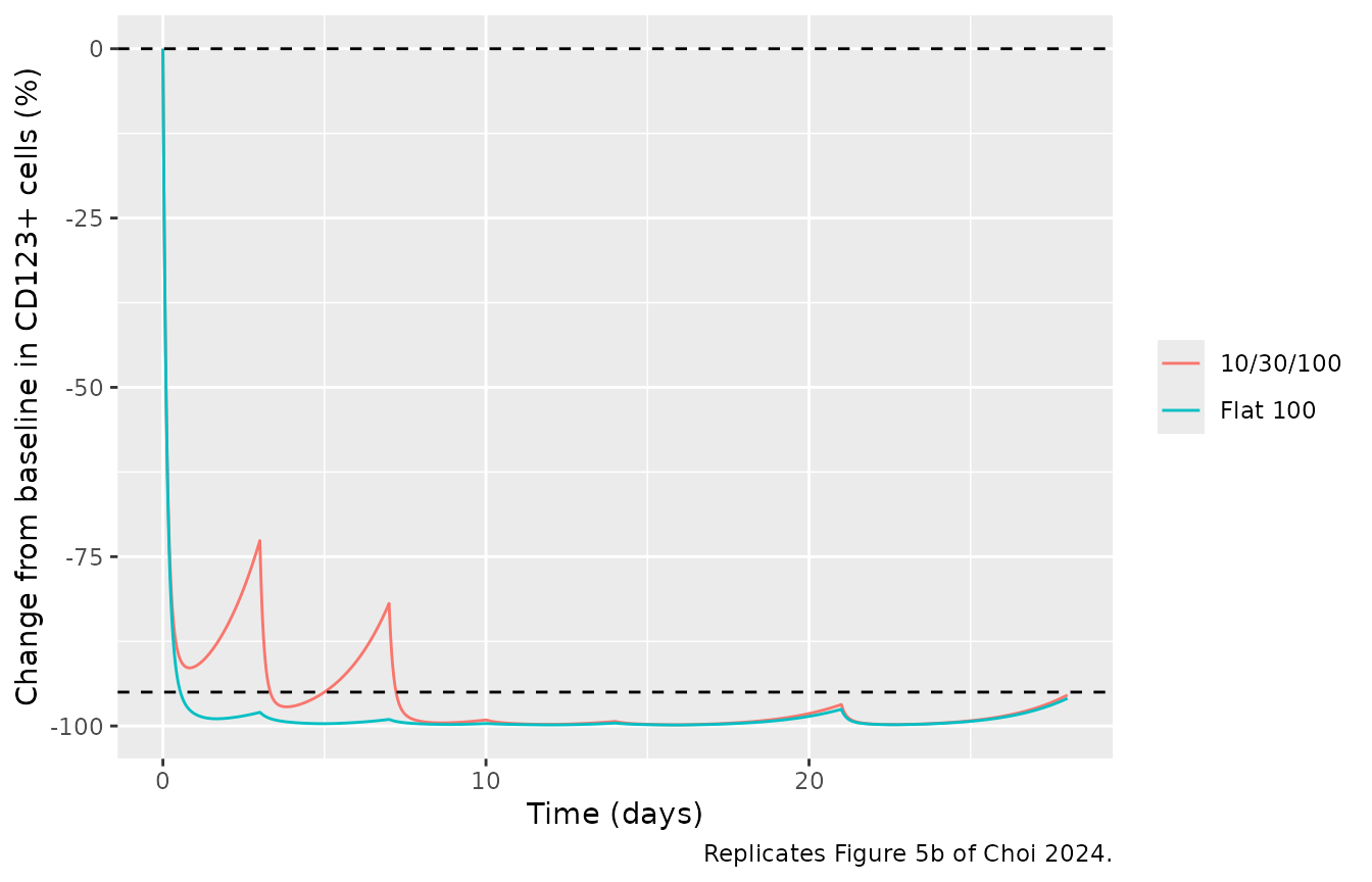
The values below are compared with readings the maintainers took from Figure 5. They are accurate to roughly a factor of 1.5 on the logarithmic PK axis and to a few percentage points on the linear change-from-baseline axis.
aml_at <- function(reg, t_h, var) {
  v <- sim_aml[[var]][sim_aml$regimen == reg & abs(sim_aml$time - t_h) < 1e-9]
  if (length(v) != 1L) stop("no unique row for ", reg, " at ", t_h, " h")
  v
}
first_peak <- function(reg) max(sim_aml$Cc[sim_aml$regimen == reg & sim_aml$time > 0 & sim_aml$time <= 2])

fig5 <- tibble::tribble(
  ~quantity, ~regimen, ~figure5, ~simulated,
  "Peak after first dose (nM)", "Flat 100", 8, first_peak("Flat 100"),
  "Peak after first dose (nM)", "10/30/100", 0.07, first_peak("10/30/100"),
  "Trough before day-3 dose (nM)", "Flat 100", 6e-3, aml_at("Flat 100", h(3) - 0.5, "Cc"),
  "Trough before day-3 dose (nM)", "10/30/100", 2e-5, aml_at("10/30/100", h(3) - 0.5, "Cc"),
  "Concentration on day 28 (nM)", "Flat 100", 1.5e-3, aml_at("Flat 100", h(28), "Cc"),
  "CD123+ change at day 1 (%)", "10/30/100", -92, aml_at("10/30/100", h(1), "cd123_pctcfb"),
  "CD123+ change before day-3 dose (%)", "10/30/100", -75, aml_at("10/30/100", h(3) - 0.5, "cd123_pctcfb"),
  "CD123+ change on day 28 (%)", "Flat 100", -96.5, aml_at("Flat 100", h(28), "cd123_pctcfb")
)
fig5 |>
  mutate(
    figure5 = vapply(figure5, \(x) format(x, trim = TRUE), character(1)),
    simulated = vapply(simulated, \(x) format(signif(x, 3), trim = TRUE), character(1))
  ) |>
  dplyr::rename("Quantity" = quantity, "Regimen" = regimen, "Figure 5" = figure5, "Simulated" = simulated) |>
knitr::kable()| Quantity | Regimen | Figure 5 | Simulated |
|---|---|---|---|
| Peak after first dose (nM) | Flat 100 | 8 | 7.96 |
| Peak after first dose (nM) | 10/30/100 | 0.07 | 0.132 |
| Trough before day-3 dose (nM) | Flat 100 | 0.006 | 0.00428 |
| Trough before day-3 dose (nM) | 10/30/100 | 2e-05 | 1.38e-05 |
| Concentration on day 28 (nM) | Flat 100 | 0.0015 | 0.0012 |
| CD123+ change at day 1 (%) | 10/30/100 | -92 | -91.2 |
| CD123+ change before day-3 dose (%) | 10/30/100 | -75 | -73 |
| CD123+ change on day 28 (%) | Flat 100 | -96.5 | -95.9 |
pk_rows <- grepl("nM", fig5$quantity)
stopifnot(
  # PK readings within a factor of 2 on the log axis
  all(abs(log(fig5$simulated[pk_rows] / fig5$figure5[pk_rows])) < log(2)),
  # Change-from-baseline readings within 5 percentage points
  all(abs(fig5$simulated[!pk_rows] - fig5$figure5[!pk_rows]) < 5)
)
The two dose-selection criteria hold as the paper reports. The flat 100 ug/kg regimen exceeds 1.7 nM at the first dose. The 10 ug/kg first dose peaks about one log unit below the threshold. Both regimens reduce CD123+ cells by more than 95% during the first cycle. “Peak” here is the highest free concentration after the first few minutes, which is what Figure 5 plots. Immediately after the bolus, before any binding, the concentration is simply dose / V1: 16 nM for 100 ug/kg and 1.6 nM for 10 ug/kg (see the NCA below). Binding to the 8.5 nM non-blood CD123 pool removes most of a 10 ug/kg dose within minutes.
cfb_min <- sim_aml |>
  group_by(regimen) |>
  summarise(nadir = min(cd123_pctcfb), day28 = cd123_pctcfb[time == h(28)], .groups = "drop")
cfb_min
#> # A tibble: 2 × 3
#>   regimen   nadir day28
#>   <chr>     <dbl> <dbl>
#> 1 10/30/100 -99.8 -95.4
#> 2 Flat 100  -99.8 -95.9
stopifnot(
  first_peak("Flat 100") > 1.7,
  first_peak("10/30/100") < 1.7 / 10,
  all(cfb_min$nadir < -95),
  all(cfb_min$day28 < -95)
)
PKNCA
The paper reports no NCA parameters, so there is no published table to compare against. The NCA below summarises the simulated exposure, grouped by arm, over the first dosing interval of each scenario. For the monkeys, that covers the single-dose arms (0-168 h, before anti-drug antibodies emerge). For the patients with AML, it is the first 72 h of each regimen, up to but not including the second dose.
nca_nhp_conc <- sim_nhp |>
  filter(arm %in% c("IV 3000 SD", "SC 3.6 SD"), time <= 168, !is.na(Cc)) |>
  select(id, time, Cc, arm)
nca_nhp_conc <- dplyr::bind_rows(
  nca_nhp_conc,
  nca_nhp_conc |> dplyr::distinct(id, arm) |> mutate(time = 0, Cc = 0)
) |>
  dplyr::distinct(id, arm, time, .keep_all = TRUE) |>
  arrange(id, arm, time)
# Concentrations may undershoot zero by integrator noise in the far tail.
stopifnot(all(nca_nhp_conc$Cc >= -1e-6 * max(nca_nhp_conc$Cc)))
nca_nhp_conc$Cc <- pmax(nca_nhp_conc$Cc, 0)

nca_nhp_dose <- nhp_events |>
  filter(evid == 1L, arm %in% c("IV 3000 SD", "SC 3.6 SD")) |>
  select(id, time, amt, arm) |>
  mutate(arm = as.character(arm))
nca_nhp_conc$arm <- as.character(nca_nhp_conc$arm)

nca_nhp <- PKNCA::pk.nca(PKNCA::PKNCAdata(
  PKNCA::PKNCAconc(nca_nhp_conc, Cc ~ time | arm + id),
  PKNCA::PKNCAdose(nca_nhp_dose, amt ~ time | arm + id),
  intervals = data.frame(start = 0, end = 168, cmax = TRUE, tmax = TRUE, auclast = TRUE)
))
nca_nhp_summary <- summary(nca_nhp)
knitr::kable(nca_nhp_summary, caption = "Simulated monkey NCA, 0-168 h (geometric mean and CV).")| start | end | arm | N | auclast | cmax | tmax |
|---|---|---|---|---|---|---|
| 0 | 168 | IV 3000 SD | 50 | 35300 [11.9] | 493 [13.7] | 1.00 [1.00, 1.00] |
| 0 | 168 | SC 3.6 SD | 50 | 0.843 [63.6] | 0.0187 [56.8] | 15.0 [12.0, 18.0] |
nca_aml_conc <- sim_aml |>
  filter(time < 72, !is.na(Cc)) |>
  select(id, time, Cc, regimen)
nca_aml_dose <- aml_events |>
  filter(evid == 1L, time == 0) |>
  select(id, time, amt, regimen)
nca_aml <- PKNCA::pk.nca(PKNCA::PKNCAdata(
  PKNCA::PKNCAconc(nca_aml_conc, Cc ~ time | regimen + id),
  PKNCA::PKNCAdose(nca_aml_dose, amt ~ time | regimen + id),
  intervals = data.frame(start = 0, end = 72, cmax = TRUE, tmax = TRUE, auclast = TRUE)
))
nca_aml_res <- as.data.frame(nca_aml$result)
nca_aml_res |>
  filter(PPTESTCD %in% c("cmax", "tmax", "auclast")) |>
  select(regimen, PPTESTCD, PPORRES) |>
  tidyr::pivot_wider(names_from = PPTESTCD, values_from = PPORRES) |>
  dplyr::rename(
    "Regimen" = regimen, "Cmax (nM)" = cmax, "Tmax (h)" = tmax,
    "AUC0-72 (nM*h)" = auclast
  ) |>
knitr::kable(digits = 3)| Regimen | AUC0-72 (nM*h) | Cmax (nM) | Tmax (h) |
|---|---|---|---|
| 10/30/100 | 0.626 | 1.598 | 0 |
| Flat 100 | 120.129 | 15.980 | 0 |
nca_val <- function(reg, param) {
  v <- nca_aml_res$PPORRES[nca_aml_res$regimen == reg & nca_aml_res$PPTESTCD == param]
  if (length(v) != 1L) stop("no unique ", param, " for ", reg)
  v
}
# Cmax is the post-bolus concentration dose * 1e3 / MW / V1.
cmax_closed <- c("Flat 100" = 100, "10/30/100" = 10) * 1e3 / 149000 / 0.042
auc_ratio <- nca_val("Flat 100", "auclast") / nca_val("10/30/100", "auclast")
auc_ratio
#> [1] 191.807
stopifnot(
  abs(nca_val("Flat 100", "cmax") / cmax_closed[["Flat 100"]] - 1) < 1e-3,
  abs(nca_val("10/30/100", "cmax") / cmax_closed[["10/30/100"]] - 1) < 1e-3,
  # Target-mediated disposition: a 10-fold dose ratio gives a much larger
  # exposure ratio.
  auc_ratio > 20
)
Cmax equals dose / V1 for both regimens, because the doses are boluses. The target-mediated sink shows in the exposure instead: a 10-fold lower first dose gives a far more than 10-fold lower AUC over the first 72 h, because the non-blood CD123 pool binds most of a small dose.
Assumptions and deviations
-
Free-CD123 term in the in vitro model. Appendix S1
Eq 10 computes total CD123 from the baseline cell count
TC0. The packaged model uses the surviving treated-cell count, as the Monolix script of the AML model does, because only that form reproduces the typical curves of Figure 3 with the published estimates (see the comparison table above). -
Printed typos corrected. In Appendix S1, Eq 3 (in
vitro
dTB/dt) haskon2*T*Eas its first term, and Eq 4 has+koff1*TBE. Both were taken in the mass-balanced forms of Table S2 (kon2*T*Band-koff1*TBE). The undefinedkinttbin the Table S2ddt_TAPline was taken askint, per Eq 17. Eq 21’s initial condition is printed asTC(0) = TC0; it is taken asM(0) = TC0, as in Table S2 (M_0 = TA0). The Results text gives a “14-h” NK half-life, but Table 1 (kout= 0.002 1/h) and the Discussion both correspond to 14 days; the Table 1 value is used. -
NK-redistribution exponent. Table S2 raises the
synapse to an exponent
nNKthat Table 1 does not list. Appendix S1 Eq 19 has no exponent, sonNK= 1. -
Monkey baselines. The paper used each animal’s
observed NK and CD123+ baseline as a regressor. The model carries the
cohort medians (247 and 28 cells/uL) as fixed parameters; set
rbase_nkandrbase_cd123per subject throughrxSolve(params = )to reproduce the individual-baseline form. Likewise, the in vitro NK concentrationrbase_nkdefaults to the 10:1 E:T arm and is set per well. -
Anti-drug antibody switch. Appendix S1 Eq 14
replaces the IV and SC inputs with 1e-9 after
TADA. The packaged model sets them to zero: doses given afterTADAdeliver nothing, and the SC depot stops feeding the central compartment. -
Monkey IV infusion and molecular weight. All monkey
IV doses were 1-h infusions (Table S1), and the simulations above use
dur = 1. The monkey PK uses the 149 kDa molecular weight of the AML script, which the paper does not restate for the monkey model. It reproduces the about 500 nM end-of-infusion concentration of Figure 4a. - Residual error. The paper does not report residual-error estimates for any of the three models, so none is included. The models simulate typical or individual predictions only. Monkey PK and CD123+ data below the limit of quantification were handled with the M3 method in the original fit.
- AML regimen schedule. Figure 5 is labelled twice weekly but draws doses on days 0, 3, 7, 10, 14 and 21; that schedule is used.
- Species label. The paper refers to the animals only as monkeys / nonhuman primates and does not name the species.