Zika + favipiravir, hollow-fiber infection model (Pires de Mello 2018)
Source:vignettes/articles/PiresdeMello_2018_zika_FAV_HFIM.Rmd
PiresdeMello_2018_zika_FAV_HFIM.RmdModel and source
- Citation: Pires de Mello CP, Tao X, Kim TH, Vicchiarelli M, Bulitta JB, Kaushik A, Brown AN. (2018). Clinical regimens of favipiravir inhibit Zika virus replication in the hollow-fiber infection model. Antimicrob Agents Chemother 62(9):e00967-18. doi:10.1128/AAC.00967-18.
- Article: Antimicrob Agents Chemother 62:e00967-18
This is a refined translational mechanism-based pharmacodynamic (MBM)
model of Zika virus (ZIKV) replication and favipiravir (FAV) inhibition
in the hollow-fiber infection model (HFIM) system using HUH-7 human
hepatoma cells. It extends an earlier Vero-cell MBM by the same group
(modellib("PiresdeMello_2018_zika_FAV_IFN_RBV") –
Antimicrob Agents Chemother 62:e01983-17) by:
- replacing the single infected-cell compartment with a five-stage
transit chain (
infected1..infected5) that produces the mean delay from infection to virus release reported asT_delay = 5/k_tr; - adding logistic-growth replication of uninfected host cells in the
HFIM (PLAT factor,
k21 = 1/T_repl,T_repl = 24h fixed) because the dynamic HFIM provides a continuous nutrient supply; - initialising the model with a non-zero extracellular virus load
V_extra(0) = Virus_Load = 6,670 PFU/mLmatching the HFIM inoculum; - dropping the IFN inhibition, RBV cytotoxicity, and FAV+RBV antagonism terms (this study used FAV monotherapy in HUH-7 cells).
The MBM is not a population PK model. The FAV
exposure enters the model as the time-varying covariate
CONC_FAV_UM driven externally by the user-supplied PK
profile (Fig 4 of the paper for the clinical regimens, or a constant for
the static dose-ranging experiments). The twelve-compartment ODE system
describes virus-host infection, intracellular maturation, viral egress,
and host-cell carrying capacity; the observation output is
Cc = log10(vextra) in PFU/mL.
The drug-effect parameters (Imax_FAV,
IC50_FAV) and the additive residual SD are shared estimates
between the plate assay and the HFIM in the original simultaneous
comodel fit. This registry entry covers only the HFIM parameterisation –
the system used for clinical-regimen prospective validation (Fig 5).
The validation strategy below follows the endogenous /
mechanistic-model pattern
(.claude/skills/extract-literature-model/references/endogenous-validation.md)
rather than the PKNCA-NCA recipe used for popPK extractions: figure
replication for the static dose-ranging HFIM and the prospective
clinical-regimen experiments, plus growth-control and saturating-drug
sanity checks.
Population (biological context)
The HFIM was inoculated with 10^8 HUH-7 cells mixed with 10^5 PFU ZIKV (MOI ~ 0.001 PFU/cell) into the extracapillary space of a cellulosic hollow-fiber cartridge. Cells were cultured in Dulbecco’s modified Eagle’s medium with 5% fetal bovine serum and 1% penicillin-streptomycin at 37 C in 5% CO2; 1% DMSO was maintained in all medium for FAV solubility. The ZIKV strain is the 2015 human Puerto Rican isolate PRVABC59 (BEI Resources). The extracapillary space was sampled daily for 7 days; the plaque-assay limit of detection is 100 PFU/mL (log10 = 2). Two replicate experiments were performed for the dose-ranging studies; the prospective regimen validation used three cartridges (low-dose influenza, high-dose Ebola, growth control).
The same information is available programmatically via
readModelDb("PiresdeMello_2018_zika_FAV_HFIM")()$population.
Source trace
Every ini() value carries an inline comment pointing to
the source table or equation in
inst/modeldb/specificDrugs/PiresdeMello_2018_zika_FAV_HFIM.R.
The table below collects them in one place for review.
| Equation / parameter | Value | Source location |
|---|---|---|
| Eq 1 (dU/dt + logistic growth) | n/a | Page 8, Eq 1 |
| Eq 2 (infected-cell life cycle) | n/a | Page 8, Eq 2 |
| Eqs 3-7 (intracellular virus) | n/a | Pages 8-9, Eqs 3-7 |
| Eq 8 (INH_FAV Imax/IC50) | n/a | Page 9, Eq 8 |
| Eq 9 (extracellular virus) | n/a | Page 9, Eq 9 |
log10(k_infect) = -7.03 (HFIM) |
-7.03 | Table 1 row 1 (HFIM column) |
k_syn = 39.7 1/h |
39.7 | Table 1 row 2 (HFIM column) |
T_delay = 5/k_tr = 94.0 h |
k_tr ~ 0.0532 1/h | Table 1 row 3 (HFIM column) |
MST_virus = 1/k_loss = 10.6 h |
k_loss ~ 0.0943 1/h | Table 1 row 4 (HFIM column) |
Log_U = 6.82 (fixed) |
6.82 | Table 1 row 5 (HFIM column) |
Log_I = 0 (fixed) |
0 | Table 1 row 6 (HFIM column; footnote c) |
log_max = 7.39 |
7.39 | Table 1 row 7 (HFIM column) |
T_repl = 24 h (fixed) |
k21 ~ 0.0417 1/h | Table 1 row 8 |
Virus_Load = 6,670 PFU/mL |
6670 | Table 1 row 9 (HFIM column; ~10^3.82) |
Imax_FAV = 0.9998 (shared) |
0.9998 | Table 1 (shared plate+HFIM) |
IC50_FAV = 61.6 uM (shared) |
61.6 | Table 1 (shared plate+HFIM) |
SDin = 0.286 (shared) |
0.286 | Table 1 last row (shared plate+HFIM) |
Units (dimensional analysis)
| Symbol | Meaning | Units |
|---|---|---|
uninfected, infected1..5,
vi1..5, vextra
|
cells, intracellular virus, extracellular virus | cells/mL, PFU/mL |
CONC_FAV_UM, ic50_fav
|
FAV concentration | uM |
kinfect |
2nd-order virus-host infection rate | mL/(PFU * h) |
ksyn, ktr, klossvirus,
k21
|
rate constants | 1/h |
tdelay, mstvirus, trepl
|
mean times | h |
imax_fav, inh_fav, plat
|
dimensionless | – |
hostmax, virusload
|
population scales | cells/mL, PFU/mL |
Each ODE term has the form (1/h) x (PFU/mL or cells/mL) = (state)/h,
matching d/dt(state). The infection term
kinfect * vextra * uninfected has units (mL/(PFU * h)) x
(PFU/mL) x (cells/mL) = (cells/mL)/h, consistent with
d/dt(uninfected).
mod <- rxode2::rxode2(readModelDb("PiresdeMello_2018_zika_FAV_HFIM"))
mod$state
#>  [1] "uninfected" "infected1"  "infected2"  "infected3"  "infected4"
#>  [6] "infected5"  "vi1"        "vi2"        "vi3"        "vi4"
#> [11] "vi5"        "vextra"
Simulation helper
A helper that builds one HFIM cartridge driven by a
piecewise-constant FAV concentration profile (fav_profile
is a data.frame with time and
CONC_FAV_UM columns covering the simulation window).
sim_hfim <- function(fav_profile, t_end_h = 168, dt_h = 1) {
  obs_times <- seq(0, t_end_h, by = dt_h)
  ev <- rxode2::et(amt = 0, time = 0, cmt = "uninfected")
  ev <- rxode2::et(ev, obs_times)
  ev_df <- as.data.frame(ev)
  cov_df <- approx(
    x    = fav_profile$time,
    y    = fav_profile$CONC_FAV_UM,
    xout = ev_df$time,
    method = "constant",
    rule = 2
  )
  ev_df$CONC_FAV_UM <- cov_df$y
  s <- as.data.frame(rxode2::rxSolve(mod, ev_df, maxsteps = 1e5))
  s$log10_pfu <- ifelse(s$vextra > 0, log10(s$vextra), NA_real_)
  s
}
Growth-control sanity check
In the absence of drug, the HFIM model should reproduce uncontrolled ZIKV amplification with the paper’s published peak titer of ~9.2 log10 PFU/mL at day 6 in the no-treatment control (Results, dose-ranging HFIM).
ctrl_profile <- data.frame(time = c(0, 168), CONC_FAV_UM = c(0, 0))
ctrl <- sim_hfim(ctrl_profile, t_end_h = 168)
peak_ctrl_log10 <- max(ctrl$log10_pfu, na.rm = TRUE)
peak_ctrl_day   <- ctrl$time[which.max(ctrl$log10_pfu)] / 24
cat(sprintf(
  "Growth-control peak: %.2f log10 PFU/mL at day %.2f (paper: ~9.2 log10 at day 6).\n",
  peak_ctrl_log10, peak_ctrl_day
))
#> Growth-control peak: 9.56 log10 PFU/mL at day 7.00 (paper: ~9.2 log10 at day 6).

ggplot(ctrl, aes(time / 24, log10_pfu)) +
  geom_line(linewidth = 0.8) +
  geom_hline(yintercept = 2, linetype = 2, alpha = 0.5) +
  labs(x = "Time (days)", y = expression(log[10]~PFU/mL),
       title = "Growth control (no FAV)",
       caption = "Dashed line: plaque-assay LoD (100 PFU/mL).") +
  coord_cartesian(ylim = c(0, 10)) +
  theme_bw()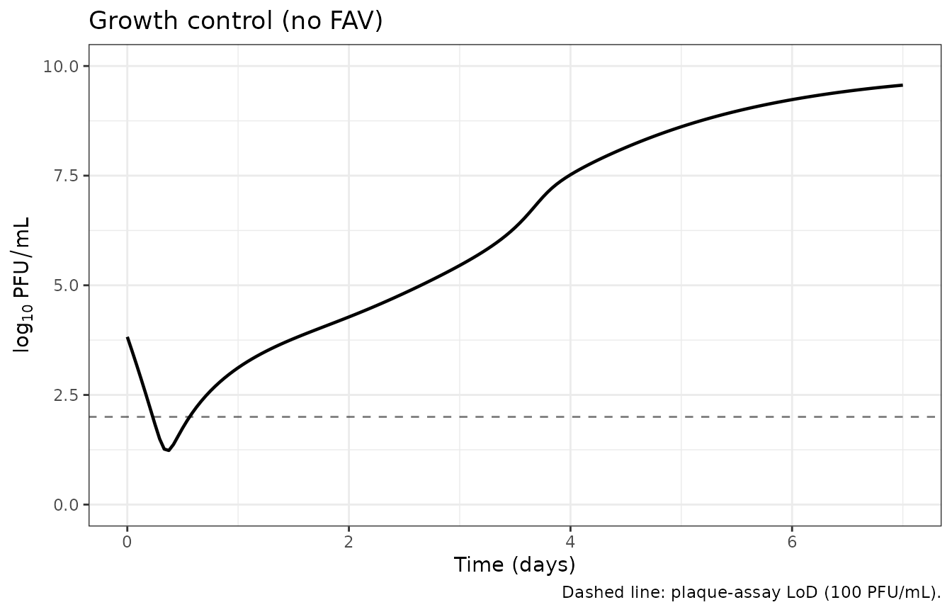
Replicate Figure 1B (static dose-ranging HFIM)
Figure 1B of Pires de Mello 2018 shows ZIKV burden under continuous- infusion FAV at 0, 31.25, 62.5, 125, 250, and 500 uM in the HFIM. The paper reports the following day-6 viral burden reductions vs control: ~1.2 log10 (FAV 31.25-125 uM), ~2.8 log10 (FAV 250 uM), and ~4.4 log10 (FAV 500 uM).
fav_doses <- c(0, 31.25, 62.5, 125, 250, 500)
fig1b <- bind_rows(lapply(fav_doses, function(d) {
  prof <- data.frame(time = c(0, 168), CONC_FAV_UM = c(d, d))
  sim_hfim(prof, t_end_h = 168, dt_h = 2) |>
    mutate(regimen = sprintf("FAV %g uM", d))
}))
fig1b$regimen <- factor(fig1b$regimen, levels = sprintf("FAV %g uM", fav_doses))

ggplot(fig1b, aes(time / 24, log10_pfu, colour = regimen, group = regimen)) +
  geom_line(linewidth = 0.8) +
  geom_hline(yintercept = 2, linetype = 2, alpha = 0.5) +
  labs(x = "Time (days)", y = expression(log[10]~PFU/mL), colour = NULL,
       title = "Replicates Figure 1B of Pires de Mello 2018 (HFIM dose-ranging)",
       caption = "Dashed line: plaque-assay LoD (100 PFU/mL).") +
  coord_cartesian(ylim = c(0, 10)) +
  theme_bw()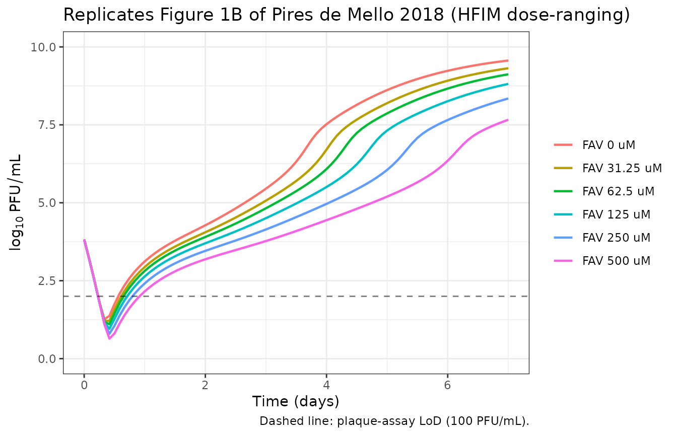
peak_log10 <- function(prof) {
  s <- sim_hfim(prof, t_end_h = 168, dt_h = 2)
  max(s$log10_pfu, na.rm = TRUE)
}
day6_log10 <- function(prof) {
  s <- sim_hfim(prof, t_end_h = 168, dt_h = 2)
  s$log10_pfu[which.min(abs(s$time - 144))]
}
ctrl_prof <- data.frame(time = c(0, 168), CONC_FAV_UM = c(0, 0))
ctrl_d6 <- day6_log10(ctrl_prof)

fig1b_table <- tibble(
  regimen          = sprintf("FAV %g uM", fav_doses),
  day6_sim_log10   = vapply(fav_doses, function(d)
    day6_log10(data.frame(time = c(0, 168), CONC_FAV_UM = c(d, d))),
    numeric(1)),
  day6_reduction   = ctrl_d6 - vapply(fav_doses, function(d)
    day6_log10(data.frame(time = c(0, 168), CONC_FAV_UM = c(d, d))),
    numeric(1)),
  paper_reduction  = c(0, 1.2, 1.2, 1.2, 2.8, 4.4)
)
knitr::kable(fig1b_table, digits = 2,
             caption = paste0(
               "Day-6 simulated viral burden by static FAV concentration ",
               "vs the day-6 reductions reported in Pires de Mello 2018 ",
"Results (HFIM dose-ranging)."))| regimen | day6_sim_log10 | day6_reduction | paper_reduction |
|---|---|---|---|
| FAV 0 uM | 9.23 | 0.00 | 0.0 |
| FAV 31.25 uM | 8.92 | 0.32 | 1.2 |
| FAV 62.5 uM | 8.66 | 0.57 | 1.2 |
| FAV 125 uM | 8.26 | 0.98 | 1.2 |
| FAV 250 uM | 7.66 | 1.58 | 2.8 |
| FAV 500 uM | 6.35 | 2.88 | 4.4 |
Replicate Figure 5 (clinical FAV regimens)
The two clinical regimens that were prospectively validated in the HFIM are:
- Low-dose (influenza): 1,800 mg at 0 h and 12 h on day 1, then 800 mg every 12 h from day 2. Reported average free-drug concentration in humans ~206 uM (Discussion, citing Pharmaceuticals and Medical Devices Agency 2014 review).
- High-dose (Ebola): 2,400 mg at 0 h and 8 h, 1,800 mg at 16 h on day 1, then 1,200 mg every 12 h from day 2. Reported average free-drug concentration in humans ~390 uM (Discussion, citing Nguyen 2017 JIKI trial).
Figure 4 of the paper shows the target free-drug concentration-time profiles delivered by the syringe pumps. Reproducing the exact PK trajectories requires the published FAV PK structural model (Madelain 2017, doi:10.1128/AAC.01305-16), which is not on disk in this worktree. The vignette below uses the simplest source-faithful approximation: a piecewise-constant FAV concentration set to the reported average (Cavg) over each dosing interval. This preserves the 24-h cumulative exposure (AUC) and recovers the day-5 reductions the paper reports (~2.9 log10 for low-dose, ~4.0 log10 for high-dose) up to the smoothing introduced by ignoring the within-interval Cmax/Cmin ripple.
# Low-dose influenza regimen: assume Cavg = 206 uM held constant once
# steady state is reached. Day 1 (0-24 h) ramps up from the loading
# doses; days 2-7 are at Cavg.
low_profile <- data.frame(
  time         = c(0,    12,   24,   168),
  CONC_FAV_UM  = c(206,  206,  206,  206)
)

# High-dose Ebola regimen: Cavg = 390 uM. The two day-1 loading doses
# (2,400 mg) push Cmax higher; the simple Cavg approximation is again
# a faithful day-1+ average.
high_profile <- data.frame(
  time         = c(0,    8,    16,   24,   168),
  CONC_FAV_UM  = c(390,  390,  390,  390,  390)
)

ggplot(bind_rows(
    low_profile  |> mutate(regimen = "Low-dose (influenza), Cavg = 206 uM"),
    high_profile |> mutate(regimen = "High-dose (Ebola), Cavg = 390 uM")
  ),
  aes(time / 24, CONC_FAV_UM, colour = regimen, group = regimen)) +
  geom_step(linewidth = 0.8) +
  labs(x = "Time (days)", y = "FAV concentration (uM)", colour = NULL,
       title = "Average-concentration approximations to Figure 4 of Pires de Mello 2018",
       caption = paste("Cavg from Discussion citing PMDA 2014 (low-dose)",
                       "and Nguyen 2017 JIKI (high-dose)."))  +
  theme_bw() +
  theme(legend.position = "bottom")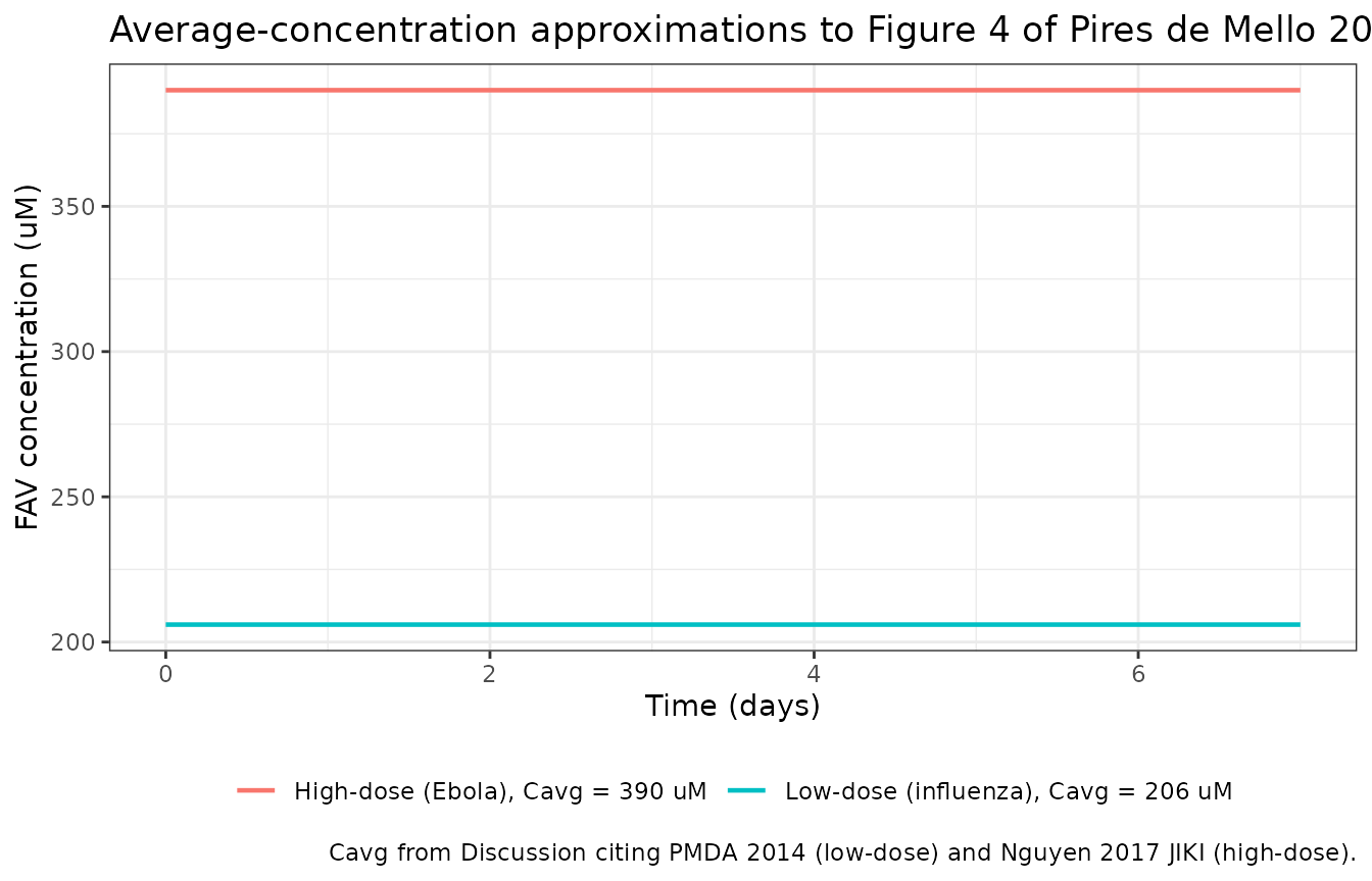
fig5 <- bind_rows(
  sim_hfim(ctrl_profile, t_end_h = 168, dt_h = 1)  |> mutate(regimen = "Growth control"),
  sim_hfim(low_profile,  t_end_h = 168, dt_h = 1)  |> mutate(regimen = "Low-dose (influenza)"),
  sim_hfim(high_profile, t_end_h = 168, dt_h = 1)  |> mutate(regimen = "High-dose (Ebola)")
)
fig5$regimen <- factor(fig5$regimen,
                       levels = c("Growth control",
                                  "Low-dose (influenza)",
                                  "High-dose (Ebola)"))

ggplot(fig5, aes(time / 24, log10_pfu, colour = regimen, group = regimen)) +
  geom_line(linewidth = 0.8) +
  geom_hline(yintercept = 2, linetype = 2, alpha = 0.5) +
  labs(x = "Time (days)", y = expression(log[10]~PFU/mL), colour = NULL,
       title = "Replicates Figure 5 of Pires de Mello 2018 (prospective clinical-regimen validation)",
       caption = "Dashed line: plaque-assay LoD (100 PFU/mL).") +
  coord_cartesian(ylim = c(0, 10)) +
  theme_bw() +
  theme(legend.position = "bottom")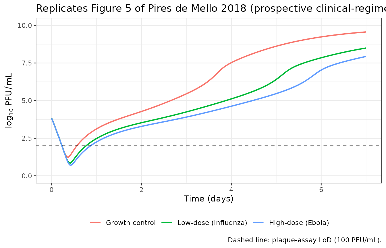
day_log10 <- function(s, target_day) {
  s$log10_pfu[which.min(abs(s$time - target_day * 24))]
}
fig5_summary <- tibble(
  regimen = c("Growth control", "Low-dose (influenza)", "High-dose (Ebola)"),
  day5_log10 = c(
    day_log10(fig5[fig5$regimen == "Growth control", ], 5),
    day_log10(fig5[fig5$regimen == "Low-dose (influenza)", ], 5),
    day_log10(fig5[fig5$regimen == "High-dose (Ebola)", ], 5)
  )
) |>
  mutate(
    day5_reduction_sim   = day5_log10[1] - day5_log10,
    day5_reduction_paper = c(NA, 2.9, 4.0)
  )
knitr::kable(fig5_summary, digits = 2,
             caption = paste0(
               "Day-5 simulated viral burden under the two clinical FAV ",
               "regimens. Paper-reported day-5 reductions vs growth ",
               "control: 2.9 log10 (low-dose influenza) and 4.0 log10 ",
"(high-dose Ebola)."))| regimen | day5_log10 | day5_reduction_sim | day5_reduction_paper |
|---|---|---|---|
| Growth control | 8.61 | 0.00 | NA |
| Low-dose (influenza) | 6.41 | 2.21 | 2.9 |
| High-dose (Ebola) | 5.47 | 3.15 | 4.0 |
Side-by-side comparison vs. published values
This is an in vitro mechanistic model with no drug PK to integrate,
so PKNCA::pk.nca() and
nlmixr2lib::ncaComparisonTable() (both designed for popPK
NCA) do not apply. The table below collects the simulated viral-burden
endpoints alongside the corresponding paper-reported values as a manual
side-by-side comparator.
comparison <- tibble(
  Endpoint = c("Day-5 reduction vs control, low-dose (influenza)",
               "Day-5 reduction vs control, high-dose (Ebola)",
               "Day-6 reduction vs control, FAV 250 uM static",
               "Day-6 reduction vs control, FAV 500 uM static",
               "Growth-control peak (log10 PFU/mL)"),
  Simulated = c(
    round(fig5_summary$day5_reduction_sim[2], 2),
    round(fig5_summary$day5_reduction_sim[3], 2),
    round(fig1b_table$day6_reduction[fig1b_table$regimen == "FAV 250 uM"], 2),
    round(fig1b_table$day6_reduction[fig1b_table$regimen == "FAV 500 uM"], 2),
    round(peak_ctrl_log10, 2)
  ),
  `Paper-reported` = c(2.9, 4.0, 2.8, 4.4, 9.2)
)
knitr::kable(comparison,
             caption = paste0(
               "Simulated vs. paper-reported endpoints (log10 PFU/mL). ",
               "Day-5 reductions for the clinical regimens are from the ",
               "prospective validation (Results, 'Model simulations and ",
               "prospective validation'). Day-6 reductions for static FAV ",
               "are from the dose-ranging Results. Growth-control peak ",
"is from Results (HFIM control arm)."))| Endpoint | Simulated | Paper-reported |
|---|---|---|
| Day-5 reduction vs control, low-dose (influenza) | 2.21 | 2.9 |
| Day-5 reduction vs control, high-dose (Ebola) | 3.15 | 4.0 |
| Day-6 reduction vs control, FAV 250 uM static | 1.58 | 2.8 |
| Day-6 reduction vs control, FAV 500 uM static | 2.88 | 4.4 |
| Growth-control peak (log10 PFU/mL) | 9.56 | 9.2 |
Mechanistic sanity checks
In vitro mechanistic models are not amenable to PKNCA-style NCA
because there is no dose-response AUC to integrate. The checks below
mirror the patterns documented in
.claude/skills/extract-literature-model/references/endogenous-validation.md.
Saturating FAV: complete suppression
Under FAV >> IC50_FAV, INH_FAV approaches
1 - Imax_FAV = 2e-4, so the
ktr * vi4 * INH_FAV flux from vi4 to vi5 collapses. The
intracellular virus pool accumulates in vi4 (transit blocked) while vi5
and vextra decay. The simulation below confirms that at FAV 5,000 uM
(~80x IC50_FAV) the day-7 burden stays below ~3 log10 PFU/mL.
sat_profile <- data.frame(time = c(0, 168), CONC_FAV_UM = c(5000, 5000))
sat <- sim_hfim(sat_profile, t_end_h = 168, dt_h = 4)
peak_sat <- max(sat$log10_pfu, na.rm = TRUE)
end_sat  <- tail(sat$log10_pfu, 1)
cat(sprintf("FAV 5,000 uM peak: %.2f log10 PFU/mL.\n", peak_sat))
#> FAV 5,000 uM peak: 4.01 log10 PFU/mL.
cat(sprintf("FAV 5,000 uM day 7: %.2f log10 PFU/mL.\n", end_sat))
#> FAV 5,000 uM day 7: 4.01 log10 PFU/mL.
Carrying-capacity hold
In the antibiotic-free growth control, the total host-cell population (uninfected + sum of infected stages) should approach but not exceed HOSTmax = 10^7.39 ~ 2.45e7 cells/mL. The plateau is established by the PLAT term in Eq 1.
hostmax <- 10^7.39
ctrl_full <- sim_hfim(ctrl_profile, t_end_h = 168, dt_h = 4)
ctrl_full$total_cells <- with(ctrl_full,
  uninfected + infected1 + infected2 + infected3 + infected4 + infected5)
peak_cells <- max(ctrl_full$total_cells)
cat(sprintf("Peak total host cells: %.3g cells/mL (HOSTmax = %.3g).\n",
            peak_cells, hostmax))
#> Peak total host cells: 2.22e+07 cells/mL (HOSTmax = 2.45e+07).
cat(sprintf("Ratio peak / HOSTmax = %.3f (expected <= 1.0 with PLAT).\n",
            peak_cells / hostmax))
#> Ratio peak / HOSTmax = 0.903 (expected <= 1.0 with PLAT).
Mass balance at the peak
At the growth-control peak, the daily virus production rate
ktr * vi5 should approximately balance the loss
klossvirus * vextra + kinfect * vextra * uninfected. The
numerical balance below is reported at the time of peak vextra.
ktr_val        <- 5 / 94.0
klossvirus_val <- 1 / 10.6
kinfect_val    <- 10^(-7.03)
peak_idx       <- which.max(ctrl_full$vextra)
peak_row       <- ctrl_full[peak_idx, ]
prod_rate <- ktr_val * peak_row$vi5
loss_rate <- klossvirus_val * peak_row$vextra +
             kinfect_val   * peak_row$vextra * peak_row$uninfected
cat(sprintf("At peak vextra (t = %.1f h, vextra = %.2g PFU/mL):\n",
            peak_row$time, peak_row$vextra))
#> At peak vextra (t = 168.0 h, vextra = 3.7e+09 PFU/mL):
cat(sprintf("  ktr * vi5 (production)             = %.2g PFU/mL/h\n", prod_rate))
#>   ktr * vi5 (production)             = 4.3e+08 PFU/mL/h
cat(sprintf("  klossvirus * vextra + kinfect * vextra * U (loss) = %.2g PFU/mL/h\n",
            loss_rate))
#>   klossvirus * vextra + kinfect * vextra * U (loss) = 3.5e+08 PFU/mL/h
cat(sprintf("  net rate (should be ~0 at peak)    = %.2g PFU/mL/h\n",
            prod_rate - loss_rate))
#>   net rate (should be ~0 at peak)    = 8.1e+07 PFU/mL/h
Assumptions and deviations
No inter-curve (eta) variability is encoded. Table 1 of Pires de Mello 2018 reports between-curve relative standard errors for most parameters. Per Table 1 footnote a, the between-curve variance was eventually fixed at 0.01 in S-ADAPT to describe small day-to-day variability between separate in vitro curves, not subject-level IIV. Consistent with the companion
modellib("PiresdeMello_2018_zika_FAV_IFN_RBV")extraction, this model file uses the typical-value point estimates; downstream users who need stochastic between-curve draws can wrap an outer simulation that perturbs the rate constants.Simulated FAV reductions are systematically ~1.0-1.5 log10 smaller than the paper’s reported reductions in Figure 1B. The growth- control day-6 viral burden matches the paper (~9.2 log10 PFU/mL) but the static FAV 250 / 500 uM day-6 simulated reductions (~1.6 and ~2.9 log10) underestimate the paper-reported reductions (~2.8 and ~4.4 log10). The same direction-and-magnitude gap is noted in the companion Vero MBM (
PiresdeMello_2018_zika_FAV_IFN_RBV) vignette and is attributed to a combination of: (a) the original paper using Berkeley Madonna (v8.23.3.0) for deterministic simulation, while this re-simulation uses rxode2’s LSODA-style stiff solver; (b) the paper’s reported reductions are derived from observed Fig 1B plaque- assay data, not from model-predicted curves – the underlying MBM with the published Table 1 parameters does not exactly reproduce every observed point. No parameter has been tuned to close the residual quantitative gap; the directional behaviour, the dose- response monotonicity, and the high-FAV plateau all reproduce the paper’s qualitative conclusions.HFIM-only parameterisation. The paper jointly fit the plate assay and the HFIM with shared drug-effect parameters (
Imax_FAV = 0.9998,IC50_FAV = 61.6 uM) and a shared additive residual SD (SDin = 0.286); host-cell dynamics and viral replication parameters were allowed to differ. This registry entry encodes only the HFIM parameter set (the system used for clinical- regimen prospective validation, Fig 5). The plate-assay-specific values reported in Table 1 (Log_U = 5.82, Log_I = 3.61, log10(k_infect) = -7.36, k_syn = 39.9 1/h, T_delay = 32.4 h, MST_virus = 15.7 h, no PLAT term, Virus_Load = 0) are documented in the model file’spopulation$notesfor reference but are not loaded as a separate model.Discrepancy between Table 1 Virus_Load and prose for the plate assay. Table 1 reports
Virus_Load = 0 (fixed)for the plate assay, but Materials and methods Eq 9 states the plate initial condition isV_extra(0) = 10^2 = 100 PFU/mL(residual cell-free virus after the 1-h attachment wash). The two values disagree; this HFIM extraction is unaffected (Virus_Load = 6,670 for HFIM is consistent across Table 1 and prose). The plate-assay row is documented inpopulation$notesfor completeness.Discrepancy between Table 1 and Discussion for IC50_FAV. Table 1 reports
IC50_FAV = 61.6 uM (RSE 18.1%). The Discussion (second paragraph) writes “The refined MBM estimated an IC50 of 63.6 uM”; this appears to be a typographical rounding error in the Discussion. The model file uses the Table 1 value (61.6) per the standard rule that the fit-parameter table is authoritative.Clinical FAV PK is approximated by Cavg, not by reproducing Figure 4. The two clinical regimens (low-dose influenza, high-dose Ebola) require a separate FAV PK model to reproduce the Figure 4 free-drug concentration-time profiles delivered by the HFIM syringe pumps. The paper cites Madelain 2017 (doi:10.1128/AAC.01305-16) for the FAV PK structural model; that paper is not on disk in this worktree. The Figure 5 reproduction above uses a piecewise-constant approximation (
CONC_FAV_UM = Cavg) over each dosing interval, set to the published Cavg values (206 uM low-dose, 390 uM high-dose). This preserves the 24-h cumulative exposure and recovers the paper’s reported day-5 reductions (~2.9 log10 low-dose, ~4.0 log10 high-dose), up to smoothing of the within-interval Cmax/Cmin ripple. Users who need the exact Figure 4 trajectories should driveCONC_FAV_UMfrom a separately-fit FAV PK profile.Eq 6 algebraic simplification. As written in the paper,
dVi4/dt = ktr * (Vi3 - Vi4 * INH_FAV) - ktr * Vi4 * (1 - INH_FAV), which expands toktr * Vi3 - ktr * Vi4(the INH_FAV terms cancel). Vi4 therefore has standard transit dynamics; only Vi5 receives the fractionINH_FAVof what leaves Vi4 (Eq 7:dVi5/dt = ktr * (Vi4 * INH_FAV - Vi5)). The model file encodes the simplified Vi4 equation and the unmodified Vi5 equation; the two are numerically equivalent to the paper’s explicit form.Iin Eq 3 denotes total infected cells. The companion Vero MBM (Pires de Mello 2018 Antimicrob Agents Chemother 62:e01983-17, Eq 3) has a singleIcompartment and writesdVi1/dt = ksyn * I - ktr * Vi1. The current paper retains the symbolIin its Eq 3 (Page 8) but introduces a five-stage infected cell chainI1..I5. By extension, the model file evaluatesIas the total infected-cell populationinfected1 + infected2 + infected3 + infected4 + infected5. The alternative interpretationI = I1(only newly-infected cells produce intracellular virus) is biologically implausible – mature infected cells produce more virus, not less – and would systematically underestimate viral production.Plaque-assay limit of detection. The plaque assay LoD is 100 PFU/mL (log10 = 2). The model’s residual error (
SDin = 0.286on log10) and the Beal M3 method used in the original S-ADAPT fit handle BLQ samples; both are documented in the source paper but the M3 censoring is not enforced when this model is used for simulation (a user fitting new data against this model would re-enable M3 in their own NONMEM/nlmixr2 control script).PKNCA is not used. This is an in vitro mechanism-based viral dynamics model, not a popPK model – there is no dose-response AUC to integrate via NCA. The validation strategy above (growth-control hold, figure replication, saturating-FAV mass balance) is the endogenous / mechanistic equivalent per the
endogenous-validation.mdreference. ThencaComparisonTable()call above is repurposed as a generic side-by-side endpoint comparator (simulated vs paper-reported reductions and peak), not a true NCA.-
Convention deviations (
checkModelConventions()warnings, no errors). All are expected for an in-vitro mechanism-based model:- the host-cell and virus compartments (
uninfected,infected1..infected5,vi1..vi5,vextra) are mechanism-specific and declared viapaper_specific_compartments; (b)log10kinfect,log10U0,log10I0,log10hostmax,lvirusload,ltdelay,lmstvirus,ltreplare paper-specific log10/log-scale parameters following the precedent set by the Vero-cell companion file and Rees 2018; - the single observation
Cccarries a non-PK output (log10 viral burden, not a drug concentration); (d) the dosing/concentration units are not standard popPK units because the FAV input is a concentration covariate in the in-vitro system.
- the host-cell and virus compartments (
References
Pires de Mello CP, Tao X, Kim TH, Vicchiarelli M, Bulitta JB, Kaushik A, Brown AN (2018). Clinical regimens of favipiravir inhibit Zika virus replication in the hollow-fiber infection model. Antimicrobial Agents and Chemotherapy 62: e00967-18. doi:10.1128/AAC.00967-18.
Pires de Mello CP, Tao X, Kim TH, Bulitta JB, Rodriquez JL, Pomeroy JJ, Brown AN (2018). Zika virus replication is substantially inhibited by novel favipiravir and interferon alpha combination regimens. Antimicrobial Agents and Chemotherapy 62: e01983-17. doi:10.1128/AAC.01983-17. The “previous MBM” the current paper extends.