Natalizumab (van den Berg 2025)
Source:vignettes/articles/vandenBerg_2025_natalizumab.Rmd
vandenBerg_2025_natalizumab.RmdModel and source
- Citation: van den Berg SPH, Toorop AA, Hooijberg F, Wolbink G, Voelkner NMF, Gelissen LMY, Killestein J, van Kempen ZLE, Dorlo TPC, Rispens T. Pharmacokinetic Model-Informed Precision Dosing of Natalizumab in Multiple Sclerosis. CPT Pharmacometrics Syst Pharmacol. 2025;14(6):1032-1041. doi:10.1002/psp4.70014
- Description: Two-compartment population PK model with parallel linear and Michaelis-Menten elimination for intravenous natalizumab in adults with relapsing-remitting multiple sclerosis on standard or extended-interval maintenance dosing, with allometric weight effects on linear clearance and central volume (van den Berg 2025)
- Article: CPT Pharmacometrics Syst Pharmacol 2025;14(6):1032-1041 (open access, PMC12167911). The Supporting Information contains the final NONMEM control stream (Section 6) and the full parameter table (Table S4).
Van den Berg et al. developed a population PK model of intravenous natalizumab, an anti-alpha4-integrin monoclonal antibody, in patients with relapsing-remitting multiple sclerosis (RRMS) on maintenance treatment, and used it to evaluate model-informed precision dosing (MIPD) of the dosing interval against a decision-tree protocol driven by therapeutic drug monitoring. The final model has two compartments with parallel linear and Michaelis-Menten (target-mediated) elimination from the central compartment. Body weight scales linear clearance and central volume as estimated power functions normalised to 70 kg; intercompartmental clearance is fixed to 0.4 L/day from an earlier natalizumab model (Muralidharan 2017).
Population
The model was fitted to 2523 serum natalizumab concentrations (2489 troughs and 34 peaks drawn 1 h after infusion) from 379 RRMS patients treated at 20 clinics in the Netherlands (van den Berg 2025 Table 1, Table S1). Median weight was 73 kg (IQR 64-83), median height 174 cm (IQR 168-180), median age 38 years (IQR 32-47), and 78.6% were female. Data were pooled from the STDMS biobank cohort (standard 4-week interval), the PDNMS trial (NCT03516526) and the two NEXTMS arms (NCT04225312) whose personalised extended intervals targeted troughs of 10 ug/mL (main) or 5 ug/mL (low). Every dose was 300 mg IV; the median dose interval was 35 days (range 21-64). Patients with anti-drug antibodies were excluded. Race was not reported.
The same information is available programmatically via
readModelDb("vandenBerg_2025_natalizumab")()$population.
Source trace
Every value is also recorded as an in-file comment next to the
matching ini() entry in
inst/modeldb/specificDrugs/vandenBerg_2025_natalizumab.R.
“Section 6” is the final-model NONMEM control stream in the Supporting
Information.
| Equation / parameter | Value | Source location |
|---|---|---|
| Two-compartment IV model, parallel linear + Michaelis-Menten elimination from central | n/a | Results “Two-Compartment PK Model”; Section 6 $DES
|
Saturable rate Vmax * C / (Km + C) with
C = A(1) / V1
|
n/a | Supplement Section 2 equation; Section 6 $DES
|
lcl |
log(0.164 L/day) | Table 2 / Table S4 CL; THETA(1) |
lvc |
log(3.48 L) | Table 2 / Table S4 Vc; THETA(2) |
lvp |
log(3.48 L) | Table 2 / Table S4 Vp; THETA(3) |
lq |
fixed(log(0.4 L/day)) | Table 2 Q (Fixed); Section 6 Q = 0.4
|
lvmax |
log(2.86 mg/day) | Table 2 / Table S4 Vmax; THETA(4) |
lkm |
log(0.875 mg/L) | Table 2 / Table S4 Km; THETA(5) |
e_wt_cl |
0.6 | Table 2 WT on CL; THETA(7) |
e_wt_vc |
0.26 | Table 2 WT on Vc; THETA(8) |
Weight form (WT/70)^theta on CL and V1 |
n/a | Table 2 footnote; Section 6 $PK
|
etalcl |
0.050678 (22.8% CV) | Table 2 IIV CL |
etalvp |
0.094605 (31.5% CV) | Table 2 IIV Vp |
etalvmax |
0.065413 (26% CV) | Table 2 IIV Vmax |
| No IIV on Vc, Q, Km | n/a | Section 6 $PK; Supplement Section 4 |
propSd |
0.22 | Table 2 proportional error 22 CV%; Section 6
W = SQRT(THETA(6)**2*IPRED**2)
|
The IIV variances use omega^2 = log(1 + CV^2). The Supplement says the CV was computed “as described elsewhere” (Mould and Upton 2012); Table S6 confirms the log-normal form, because its mean cross-validation variances (0.0512, 0.102, 0.0652) give exactly the cross-validation CVs printed in Table 2 (22.9%, 32.8%, 26.0%) under that formula.
cv_from_omega <- function(omega2) 100 * sqrt(exp(omega2) - 1)
xval <- tibble(
  Parameter = c("CL", "Vp", "Vmax"),
  `Table S6 mean omega^2` = c(0.0512, 0.102, 0.0652),
  `Table 2 cross-validation CV%` = c(22.9, 32.8, 26.0)
) |>
  mutate(`CV% from omega^2` = cv_from_omega(`Table S6 mean omega^2`))
knitr::kable(xval, digits = 2)| Parameter | Table S6 mean omega^2 | Table 2 cross-validation CV% | CV% from omega^2 |
|---|---|---|---|
| CL | 0.05 | 22.9 | 22.92 |
| Vp | 0.10 | 32.8 | 32.77 |
| Vmax | 0.07 | 26.0 | 25.96 |
Weight effect sizes
The paper reports that weight changes clearance by a factor of 0.85-1.34 and central volume by 0.93-1.14 between the 2.5th and 97.5th weight percentiles (Results). Inverting each ratio through its own exponent must recover the same pair of weights for both parameters if the two exponents were transcribed correctly.
mod <- readModelDb("vandenBerg_2025_natalizumab")
ini_vals <- rxode2::rxode(mod)$theta
#> ℹ parameter labels from comments will be replaced by 'label()'
wt_from_ratio <- function(ratio, exponent) 70 * ratio^(1 / exponent)
eff <- tibble(
  Percentile = c("2.5th", "97.5th"),
  `CL ratio` = c(0.85, 1.34),
  `Vc ratio` = c(0.93, 1.14)
) |>
  mutate(
    `Weight implied by CL (kg)` = wt_from_ratio(`CL ratio`, ini_vals[["e_wt_cl"]]),
    `Weight implied by Vc (kg)` = wt_from_ratio(`Vc ratio`, ini_vals[["e_wt_vc"]])
  )
knitr::kable(eff, digits = 2)| Percentile | CL ratio | Vc ratio | Weight implied by CL (kg) | Weight implied by Vc (kg) |
|---|---|---|---|---|
| 2.5th | 0.85 | 0.93 | 53.39 | 52.95 |
| 97.5th | 1.34 | 1.14 | 114.01 | 115.87 |
Linear and saturable clearance
At concentrations well below Km the saturable pathway clears Vmax / Km = 3.27 L/day, about twenty times the linear clearance, which is the paper’s statement that “nonlinear elimination is the dominant clearance pathway at lower concentrations” (Discussion).
cl_conc <- tibble(conc = 10^seq(-2, 2.2, length.out = 200)) |>
  mutate(
    Linear = exp(ini_vals[["lcl"]]),
    Saturable = exp(ini_vals[["lvmax"]]) / (exp(ini_vals[["lkm"]]) + conc),
    Total = Linear + Saturable
  ) |>
  pivot_longer(-conc, names_to = "pathway", values_to = "cl")

ggplot(cl_conc, aes(conc, cl, linetype = pathway)) +
  geom_line() +
  geom_vline(xintercept = c(2, 10), colour = "grey60") +
  scale_x_log10() +
  scale_y_log10() +
  labs(x = "Natalizumab concentration (ug/mL)", y = "Clearance (L/day)", linetype = NULL) +
  theme_bw()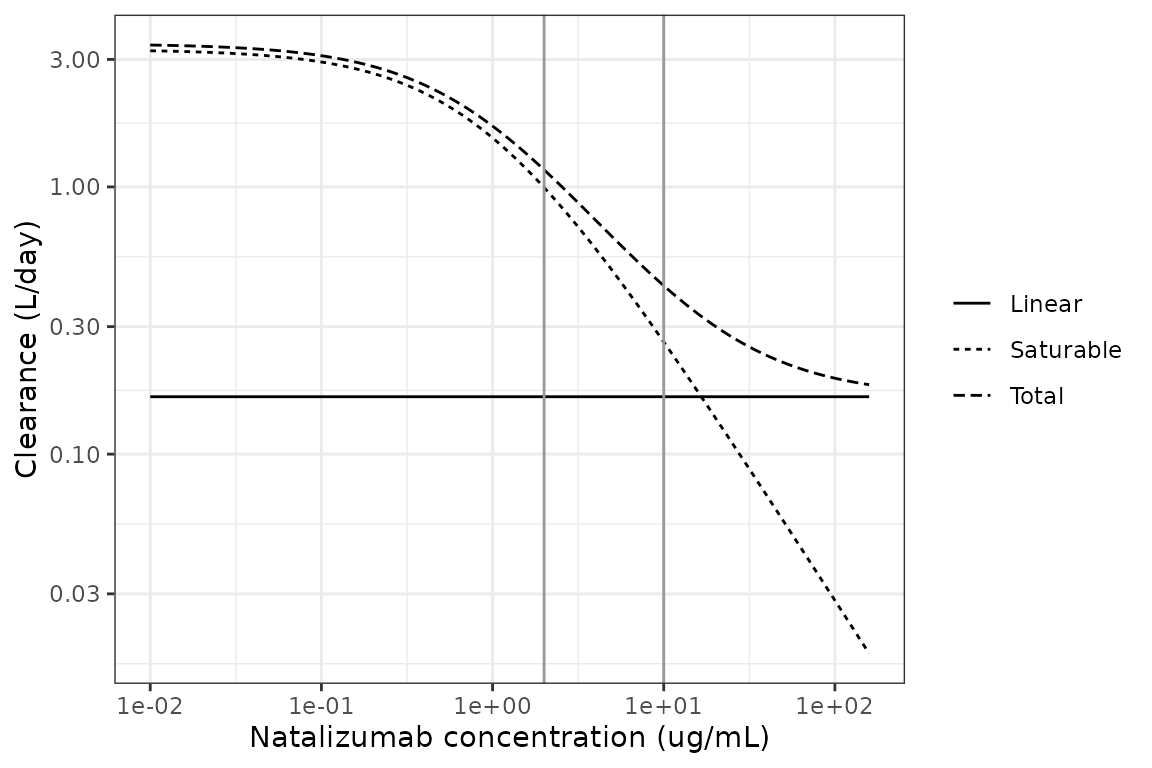
Typical linear, saturable and total clearance against serum natalizumab concentration for a 70-kg patient.
Virtual cohort
Observed data are not public. The virtual cohort draws body weight from a normal distribution with the published median (73 kg) and a standard deviation that reproduces the published IQR (64-83 kg), truncated to 40-140 kg. Between-subject random effects are drawn in base R from the published variances so that each virtual patient keeps the same individual parameters across every dosing interval simulated below, which is what the paper’s MIPD analysis does with its empirical Bayes estimates.
Each patient receives 300 mg as a 1-h IV infusion (infusion duration is not stated in the paper; 1 h is the labelled duration) for 20 doses at each whole- week interval from 4 to 12 weeks, which brings every interval to steady state (the terminal half-life of the linear pathway is about a month). Concentrations are recorded daily over the last interval and 1 h after the end of the last infusion (the paper’s peak sampling time).
set.seed(2025)
n_sub <- 200
n_dose <- 20
intervals_wk <- 4:12

omega <- c(etalcl = 0.050678, etalvp = 0.094605, etalvmax = 0.065413)
stopifnot(all(abs(omega - diag(rxode2::rxode(mod)$omega)[names(omega)]) < 1e-9))
#> ℹ parameter labels from comments will be replaced by 'label()'

wt_sd <- (83 - 64) / (2 * qnorm(0.75))
patients <- tibble(
  patient = seq_len(n_sub),
  WT = pmin(pmax(rnorm(n_sub, 73, wt_sd), 40), 140),
  etalcl = rnorm(n_sub, 0, sqrt(omega[["etalcl"]])),
  etalvp = rnorm(n_sub, 0, sqrt(omega[["etalvp"]])),
  etalvmax = rnorm(n_sub, 0, sqrt(omega[["etalvmax"]]))
)

# One rxode2 subject per patient x interval; ids ascend so the params rows
# below line up with the subjects (rxSolve matches params rows by position).
design <- tidyr::expand_grid(interval_wk = intervals_wk, patient = patients$patient) |>
  left_join(patients, by = "patient") |>
  mutate(id = row_number(), tau = 7 * interval_wk)

make_events <- function(id, tau, WT) {
  last <- (n_dose - 1) * tau
  dose <- tibble(
    id = id, time = (seq_len(n_dose) - 1) * tau, evid = 1L, amt = 300,
    rate = 300 * 24, cmt = "central"
  )
  obs <- tibble(
    id = id, time = sort(unique(c(last + 0:tau, last + 2 / 24))), evid = 0L,
    amt = 0, rate = 0, cmt = "central"
  )
  bind_rows(dose, obs) |> mutate(WT = WT)
}

events <- bind_rows(Map(make_events, design$id, design$tau, design$WT)) |>
  arrange(id, time, desc(evid))
stopifnot(!anyDuplicated(unique(events[, c("id", "time", "evid")])))
Simulation
params <- design |> select(etalcl, etalvp, etalvmax)
# All randomness (weights, etas, residual draws) comes from base R, so the
# cohort is identical on every machine. The random effects enter through
# `params`; rxode2's "multi-subject simulation without omega" warning for the
# zeroRe() model is therefore expected and silenced.
sim <- suppressWarnings(rxode2::rxSolve(
  rxode2::zeroRe(mod), events = events, params = params,
  returnType = "data.frame"
)) |>
  left_join(design |> select(id, patient, interval_wk, tau), by = "id") |>
  mutate(tad = time - (n_dose - 1) * tau)
#> ℹ parameter labels from comments will be replaced by 'label()'

# Residual-error draw (proportional, 22% CV) for the "observed" troughs.
troughs <- sim |>
  filter(tad == tau) |>
  select(id, patient, interval_wk, ipred = Cc) |>
  arrange(id) |>
  mutate(obs = ipred * (1 + ini_vals[["propSd"]] * rnorm(n())))
Steady-state troughs against Table S1
Table S1 reports the median (IQR) trough at the standard 4-week interval as 22 (15-33) ug/mL. The extended-interval troughs (median 9.9 ug/mL at a median of 42 days, and 7.6 ug/mL in the NEXTMS low arm, also at 42 days) come from patients whose interval was extended because their 4-week troughs were high, so an unselected virtual cohort dosed every 6 weeks should sit below them; they are shown for orientation and are not a gate.
trough_summary <- troughs |>
  filter(interval_wk %in% c(4, 6)) |>
  group_by(interval_wk) |>
  summarise(
    median = median(obs),
    q25 = quantile(obs, 0.25),
    q75 = quantile(obs, 0.75),
    .groups = "drop"
  ) |>
  mutate(
    published = c("22 (15-33)", "9.9 (6.9-14); selected patients"),
    simulated = sprintf("%.1f (%.1f-%.1f)", median, q25, q75)
  )
trough_summary |>
  select(interval_wk, simulated, published) |>
  rename(
    "Interval (weeks)" = interval_wk,
    "Simulated trough, median (IQR), ug/mL" = simulated,
    "Table S1 trough, median (IQR), ug/mL" = published
  ) |>
knitr::kable()| Interval (weeks) | Simulated trough, median (IQR), ug/mL | Table S1 trough, median (IQR), ug/mL |
|---|---|---|
| 4 | 24.3 (18.7-33.3) | 22 (15-33) |
| 6 | 6.5 (3.4-11.5) | 9.9 (6.9-14); selected patients |
# A mis-transcribed CL, Vmax, Km or volume moves the 4-week median trough by
# far more than this; the 25% envelope admits cohort-to-cohort noise and the
# fact that the published median pools three studies.
stopifnot(abs(trough_summary$median[1] / 22 - 1) < 0.25)
ggplot(troughs, aes(factor(interval_wk), obs)) +
  geom_boxplot(outlier.size = 0.5) +
  geom_hline(yintercept = c(10, 5, 2), colour = "grey50", linetype = "dashed") +
  scale_y_log10() +
  labs(x = "Dosing interval (weeks)", y = "Steady-state trough (ug/mL)") +
  theme_bw()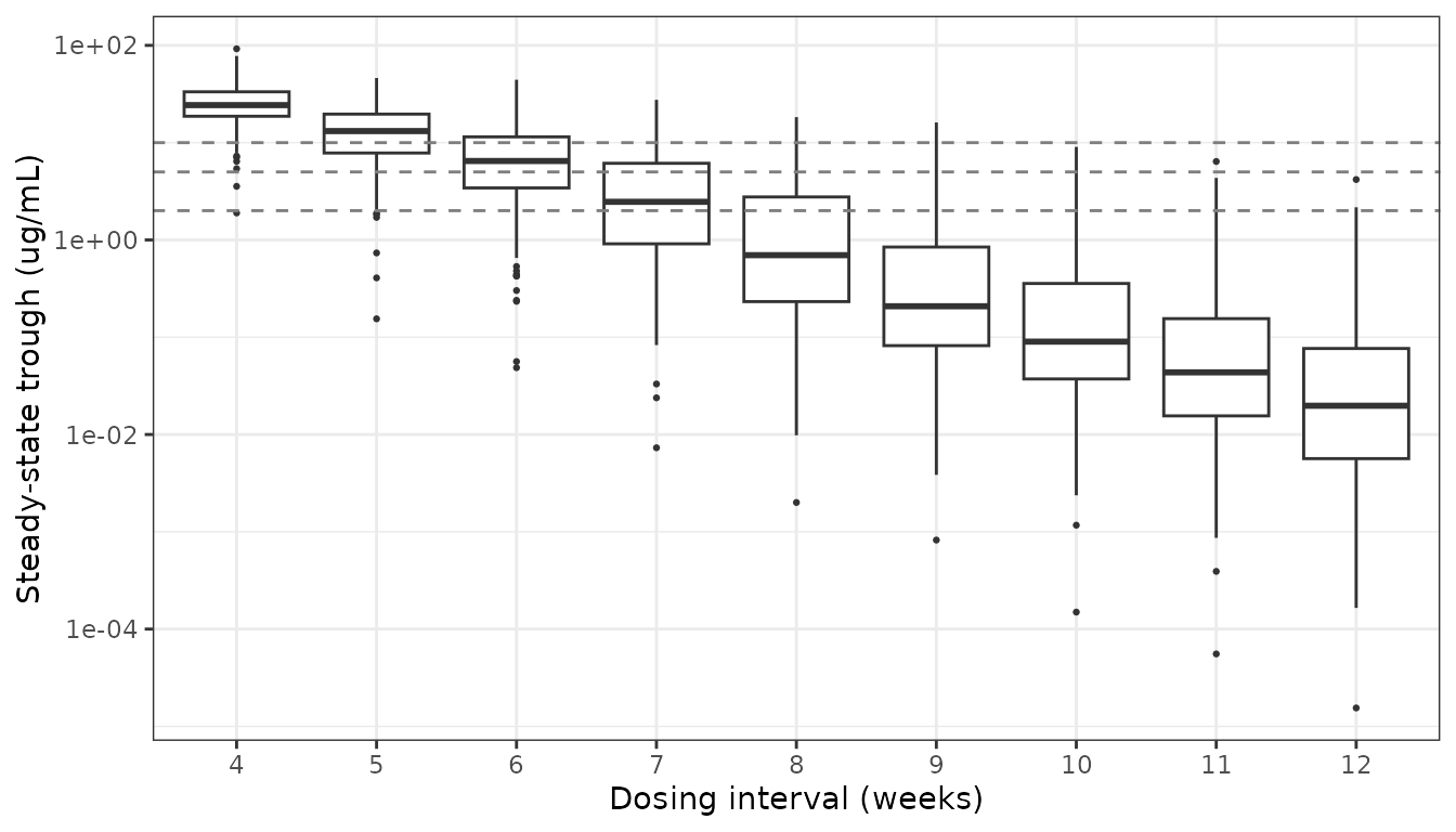
Simulated steady-state troughs (with residual error) by dosing interval. Grey lines mark the 10, 5 and 2 ug/mL targets of the paper.
PKNCA validation
PKNCA is run on the final (steady-state) interval of the 4- and
6-week regimens. The paper reports no NCA, so the comparison table uses
the only summary it gives: the median trough (cmin) at the
standard interval and the selected extended-interval median from Table
S1. ncaComparisonTable() pools by the median.
sim_nca <- sim |>
  filter(interval_wk %in% c(4, 6), !is.na(Cc)) |>
  mutate(treatment = paste0("Q", interval_wk, "W")) |>
  select(id, treatment, tad, Cc)

dose_nca <- sim_nca |>
  distinct(id, treatment) |>
  mutate(tad = 0, amt = 300)

conc_obj <- PKNCA::PKNCAconc(sim_nca, Cc ~ tad | treatment + id)
dose_obj <- PKNCA::PKNCAdose(dose_nca, amt ~ tad | treatment + id)
intervals <- data.frame(
  start = 0, end = c(28, 42), treatment = c("Q4W", "Q6W"),
  cmax = TRUE, cmin = TRUE, auclast = TRUE, cav = TRUE
)
nca_res <- PKNCA::pk.nca(PKNCA::PKNCAdata(conc_obj, dose_obj, intervals = intervals))
knitr::kable(summary(nca_res), caption = "Steady-state NCA over the final dosing interval (geometric mean and CV unless stated).")| start | end | treatment | N | auclast | cmax | cmin | cav |
|---|---|---|---|---|---|---|---|
| 0 | 28 | Q4W | 200 | 1320 [26.6] | 110 [12.1] | 23.7 [51.9] | 47.1 [26.6] |
| 0 | 42 | Q6W | 200 | 1100 [28.3] | 92.8 [9.06] | 5.65 [150] | 26.3 [28.3] |
published <- tibble::tribble(
  ~treatment, ~cmin,
  "Q4W",      22,
  "Q6W",      9.9
)
cmp <- nlmixr2lib::ncaComparisonTable(
  simulated = nca_res,
  reference = published,
  by = "treatment",
  units = c(cmax = "ug/mL", cmin = "ug/mL", auclast = "day*ug/mL", cav = "ug/mL"),
  tolerance_pct = 20
)
knitr::kable(cmp, caption = "Simulated steady-state NCA (median) vs. Table S1 trough medians. * differs from reference by >20%.")| NCA parameter | treatment | Reference | Simulated | % diff |
|---|---|---|---|---|
| Cmin (ug/mL) | Q4W | 22 | 24.3 | +10.4% |
| Cmin (ug/mL) | Q6W | 9.9 | 6.71 | -32.2%* |
The 4-week cmin agrees with the Table S1 median. The
6-week row is expected to differ: the published value describes patients
selected for extension by high 4-week troughs, while every virtual
patient here is extended regardless. The NEXTMS protocol, for example,
put a patient on a 6-week interval only after two 4-week troughs of at
least 30 ug/mL (main arm) or 25 ug/mL (low arm).
Model-informed interval selection (Figure 3)
The paper simulated four MIPD algorithms on the NEXTMS patients, choosing for each patient the whole-week interval whose individual predicted trough is closest (on the log scale) to the target; algorithms 1 and 3 accept only intervals whose predicted trough stays at or above the target. The same rules are applied here to the individual predicted troughs of the virtual cohort, with intervals limited to 4-12 weeks.
algorithms <- tibble(
  algorithm = c("A1", "A2", "A3", "A4"),
  target = c(5, 5, 2, 2),
  constrained = c(TRUE, FALSE, TRUE, FALSE)
)

pick_interval <- function(ipred, interval_wk, target, constrained) {
  dist <- abs(log(ipred) - log(target))
  ok <- if (constrained) ipred >= target else rep(TRUE, length(ipred))
  if (!any(ok)) {
    return(min(interval_wk))
  }
  interval_wk[ok][which.min(dist[ok])]
}

chosen <- tidyr::expand_grid(algorithms, patient = patients$patient) |>
  rowwise() |>
  mutate(interval_wk = {
    p <- troughs[troughs$patient == patient, ]
    pick_interval(p$ipred, p$interval_wk, target, constrained)
  }) |>
  ungroup() |>
  left_join(troughs |> select(patient, interval_wk, ipred, obs), by = c("patient", "interval_wk"))

mipd_summary <- chosen |>
  group_by(algorithm, target, constrained) |>
  summarise(
    mean_interval_wk = mean(interval_wk),
    infusions_pppy = mean(52 / interval_wk),
    pct_obs_below_target = 100 * mean(obs < target),
    .groups = "drop"
  ) |>
  mutate(reduction_pct = 100 * (1 - infusions_pppy / 13))
mipd_summary |>
  rename(
    "Algorithm" = algorithm,
    "Target (ug/mL)" = target,
    "Limit constrained" = constrained,
    "Mean interval (weeks)" = mean_interval_wk,
    "Infusions per person-year" = infusions_pppy,
    "Simulated troughs below target (%)" = pct_obs_below_target,
    "Reduction vs. 4-weekly (%)" = reduction_pct
  ) |>
knitr::kable(digits = 1)| Algorithm | Target (ug/mL) | Limit constrained | Mean interval (weeks) | Infusions per person-year | Simulated troughs below target (%) | Reduction vs. 4-weekly (%) |
|---|---|---|---|---|---|---|
| A1 | 5 | TRUE | 6.1 | 8.9 | 17.0 | 31.3 |
| A2 | 5 | FALSE | 6.5 | 8.3 | 51.5 | 36.1 |
| A3 | 2 | TRUE | 7.0 | 7.8 | 11.5 | 39.9 |
| A4 | 2 | FALSE | 7.5 | 7.2 | 56.0 | 44.5 |
chosen |>
  count(algorithm, interval_wk) |>
  group_by(algorithm) |>
  mutate(pct = 100 * n / sum(n)) |>
  ggplot(aes(factor(interval_wk), pct, fill = algorithm)) +
  geom_col(position = position_dodge(preserve = "single")) +
  labs(x = "Personalised interval (weeks)", y = "Population (%)", fill = NULL) +
  theme_bw()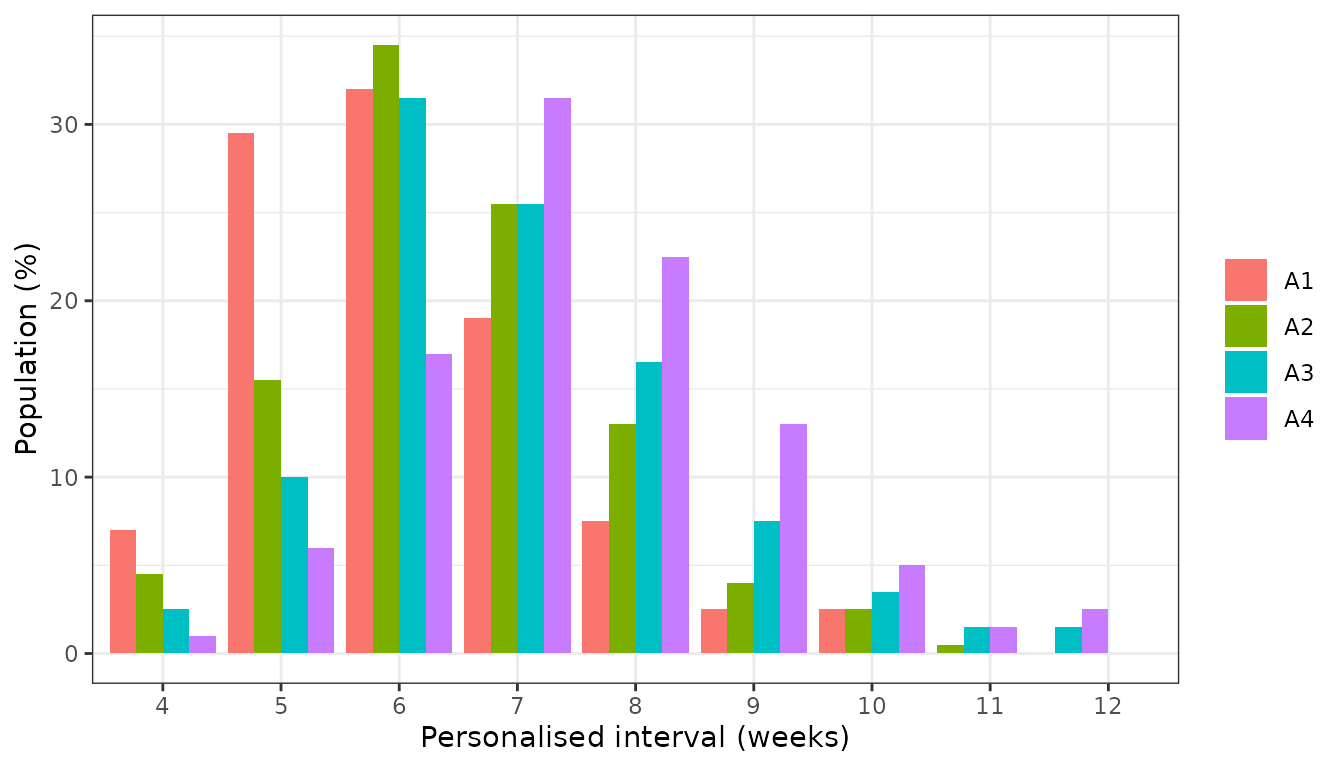
Replicates Figure 3A of van den Berg 2025: share of the population on each personalised interval under algorithms A1-A4.
ggplot(chosen, aes(algorithm, obs)) +
  geom_boxplot(outlier.size = 0.5) +
  geom_hline(yintercept = c(5, 2, 1), colour = "grey50", linetype = "dashed") +
  scale_y_log10() +
  labs(x = NULL, y = "Simulated trough (ug/mL)") +
  theme_bw()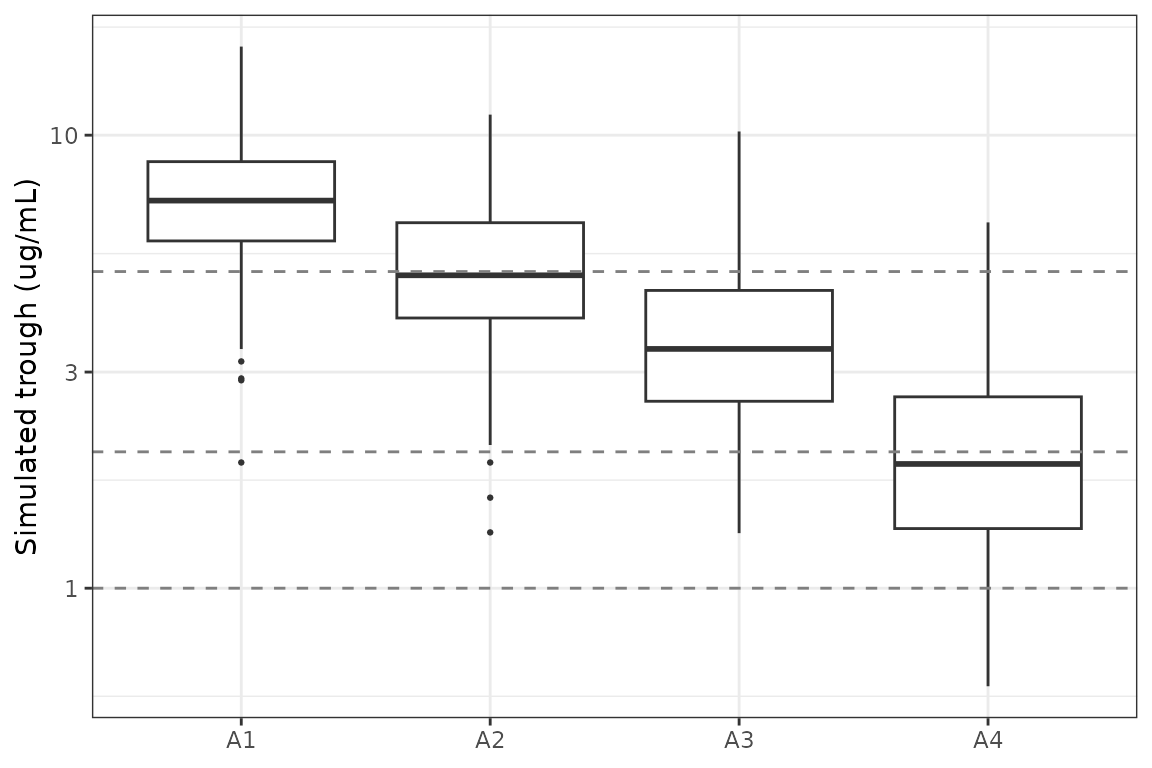
Replicates Figure 3B of van den Berg 2025: simulated observed troughs at the personalised interval under each algorithm.
The paper reports that algorithm 3 (2 ug/mL target, limit constrained) reduces infusions by 39% to about eight per person-year, with intervals of 4-10 weeks (average about 7 weeks) and 11% of patients with simulated observed troughs below 2 ug/mL, and that algorithm 2 (5 ug/mL target) reduces infusions by 35%.
a2 <- mipd_summary[mipd_summary$algorithm == "A2", ]
a3 <- mipd_summary[mipd_summary$algorithm == "A3", ]
# Means and shares over 200 patients; a mis-specified clearance pathway shifts
# the chosen intervals by whole weeks and the reductions by well over 10 points.
stopifnot(
  abs(a3$reduction_pct - 39) < 10,
  abs(a2$reduction_pct - 35) < 10,
  abs(a3$mean_interval_wk - 7) < 1,
  abs(a3$pct_obs_below_target - 11) < 8
)
Assumptions and deviations
- Infusion duration. Not stated in the paper; 1 h (the labelled duration of the 300 mg infusion) is used. Steady-state troughs are insensitive to it.
- Virtual cohort. Body weight is drawn from a normal distribution matched to the Table 1 median and IQR; no other covariate enters the model. The paper’s MIPD analysis used empirical Bayes estimates of real patients fitted to two 4-week troughs, whereas this vignette draws individual parameters from the population distribution. Because shrinkage on Vp and Vmax was high (66.7% and 35%), the paper’s individual estimates are less dispersed than the population draws, so the interval distributions in Figure 3A are only approximately reproduced.
- Residual error on the MIPD troughs. The paper drew “observed” troughs by multiplying predictions by a sampled log prediction-to-observation ratio (mean 0.02, SD 0.32; Figure S7). The model’s own 22% proportional error is used here instead.
- Clearance units in the text. The Results compare the final clearance with an earlier model as “0.164 vs. 0.15 L/h”; Table 2, Table S4 and the NONMEM code all give clearance in L/day, which is used.
- Extended-interval comparison. The 6-week rows of the trough and NCA tables are expected to fall below Table S1 because the published extended-interval patients were selected for high troughs (see above).
- No erratum or correction notice was found for this article (checked 2026-11-04).