Alectinib, crizotinib, erlotinib and gefitinib in NSCLC cell lines (Wanika 2024)
Source:vignettes/articles/Wanika_2024_tki_nsclc_invitro.Rmd
Wanika_2024_tki_nsclc_invitro.RmdModel and source
- Citation: Wanika L, Evans ND, Johnson M, Tomkinson H, Chappell MJ. In vitro PK/PD modeling of tyrosine kinase inhibitors in non-small cell lung cancer cell lines. Clin Transl Sci. 2024;17(3):e13714.
- Article: https://doi.org/10.1111/cts.13714 (open access, PMC10933606)
Wanika and co-workers built one mechanistic in vitro PK/PD model for four tyrosine kinase inhibitors (TKIs) used in non-small cell lung cancer (NSCLC) and fitted it separately to each drug in Monolix, using concentration-viability curves digitised from published 72-h cell-viability studies. The drug is added to the culture medium at time zero, exchanges first-order with the pooled intracellular space, and the intracellular concentration inhibits the production of viable tumour cells. The four fits share one structure and one vignette, and are packaged as four model files:
| Model file | Drug | Cell lines | Curves | Source |
|---|---|---|---|---|
Wanika_2024_alectinib |
alectinib | 10 | 120 | Eqs 1-5, Table 2, Table S1 |
Wanika_2024_crizotinib |
crizotinib | 11 | 129 | Eqs 1-5, Table 2, Table S2 |
Wanika_2024_erlotinib |
erlotinib | 6 | 61 | Eqs 1-5, Table 2, Table S3 |
Wanika_2024_gefitinib |
gefitinib | 5 | 82 | Eqs 1-5, Table 2, Table S4 |
drugs <- c("alectinib", "crizotinib", "erlotinib", "gefitinib")
mods <- lapply(setNames(drugs, drugs), function(d) {
  rxode2::rxode(readModelDb(paste0("Wanika_2024_", d)))
})
#> ℹ parameter labels from comments will be replaced by 'label()'
#> ℹ parameter labels from comments will be replaced by 'label()'
#> ℹ parameter labels from comments will be replaced by 'label()'
#> ℹ parameter labels from comments will be replaced by 'label()'
mods_typ <- lapply(mods, rxode2::zeroRe)
Model structure
With medium and intracellular the drug
concentrations (umol/L) and viability the tumour cell
viability (%), the paper’s Eqs 1-5 are
where
and
are the paper’s
and
(k_medium_intracellular and
k_intracellular_medium in the model files) and
is vr. Substituting Eq 5 into Eqs 1-2 gives
, so the absolute
initial cell volume
cancels and is not needed as an input, although the paper tabulates it
per curve. Because the transfer terms are scaled by the volume ratio,
the exchange itself conserves drug amount. Eq 2 has no dilution term for
the shrinking cell volume, however, so drug held in cells that are lost
as viability falls leaves the system:
.
and
are not estimated. The paper states that only
,
and
are known and supplies, for every curve, the
and
reported by the source study for that cell line. They are therefore
covariate columns, IC50_VIABILITY (umol/L) and
IMAX_VIABILITY (fraction), and must be supplied by the user
for every simulated curve.
Population
There are no subjects in the clinical sense. Each “individual” in the
Monolix fits is one concentration level of one digitised
concentration-viability curve, taken with WebPlotDigitizer from eight
(alectinib), nine (crizotinib) or seven (erlotinib, gefitinib) published
studies, with a 100% viability record at time zero and one viability
observation after 72 h of exposure (supplementary Tables S1-S4). The
cell lines are ALK-rearranged (H3122, H228, the A925 family, LC-2 ad),
EGFR-mutant (HCC827, PC9, H1975, H1650) and EGFR/ALK wild-type (A549,
H460, H1299, H292 and others) NSCLC lines, so the between-“subject”
variability spans cell line, laboratory and assay. The same information
is stored in each model’s population metadata.
Source trace
| Item | Value | Source |
|---|---|---|
| Medium / intracellular exchange | ODEs above | Eqs 1-2 (directions read from the article’s MathML) |
| Cell volume follows viability | Eq 3 | |
| Viability indirect response with Imax inhibition | ODE above | Eq 4 |
| Medium volume | Eq 5 | |
| Initial conditions | medium = dose, intracellular = 0, viability = 100% | Table 1 |
IC50_VIABILITY, IMAX_VIABILITY per
curve |
data columns | Tables S1-S4 |
| Residual error | constant (additive), | Eq 9, Table 2 |
lk_medium_intracellular (KDRUGIN) |
0.745 / 0.672 / 0.987 / 0.856 1/h | Table 2 |
lk_intracellular_medium (KDRUGOUT) |
0.096 / 0.298 / 0.051 / 0.313 1/h | Table 2 |
lvr (VR) |
4.051 / 4.234 / 3.739 / 3.192 | Table 2 |
lkin (KIN) |
1.061 / 1.126 / 2.925 / 0.941 %/h | Table 2 |
lkout (KOUT) |
0.021 / 0.026 / 0.033 / 0.034 1/h | Table 2 |
| IIV variances (KDRUGIN, KDRUGOUT, VR, KIN, KOUT) | alectinib 0.231, 0.112, 0.0348, 0.411, 0.082 | Table 2 |
| crizotinib 0.164, 0.052, 0.100, 0.205, 0.931 | Table 2 | |
| erlotinib 0.185, 0.362, 0.178, 0.067, 0.328 | Table 2 | |
| gefitinib 0.113, 0.355, 0.198, 0.068, 0.760 | Table 2 | |
addSd_viability (a) |
16.196 / 0.0136 / 0.003 / 0.737 % | Table 2 |
Values are listed in the order alectinib / crizotinib / erlotinib / gefitinib.
Data
The 72-h observations and the per-curve inputs below are transcribed from supplementary Tables S1-S4 of the paper (columns: drug initial, curve ID, cell line, source-study reference number, medium concentration in umol/L, IC50 in umol/L, IMAX as a fraction, observed viability at 72 h in %).
curves <- read.csv(
  header = FALSE,
  col.names = c("drug", "ID", "cell", "ref", "conc", "IC50_VIABILITY", "IMAX_VIABILITY", "obs"),
  text = "
a,1,H3122,1,3e-04,0.0102,0.95676,90.579
a,2,H3122,1,0.001,0.0102,0.95676,85.199
a,3,H3122,1,0.003,0.0102,0.95676,74.415
a,4,H3122,1,0.01,0.0102,0.95676,50.927
a,5,H3122,1,0.03,0.0102,0.95676,29.6
a,6,H3122,1,0.1,0.0102,0.95676,20.168
a,7,H3122,1,0.3,0.0102,0.95676,17.76
a,8,H3122,1,1,0.0102,0.95676,16.436
a,9,H3122,1,3,0.0102,0.95676,13.219
a,10,H3122,1,10,0.0102,0.95676,4.3243
a,11,A549,1,3e-04,5.52,0.67297,98.144
a,12,A549,1,0.001,5.52,0.67297,104.66
a,13,A549,1,0.003,5.52,0.67297,103.06
a,14,A549,1,0.01,5.52,0.67297,105.79
a,15,A549,1,0.03,5.52,0.67297,102.3
a,16,A549,1,0.1,5.52,0.67297,107.19
a,17,A549,1,0.3,5.52,0.67297,97.759
a,18,A549,1,1,5.52,0.67297,76.705
a,19,A549,1,3,5.52,0.67297,67.81
a,20,A549,1,10,5.52,0.67297,32.703
a,21,H460,1,3e-04,7.38,0.65459,99.461
a,22,H460,1,0.001,7.38,0.65459,97.877
a,23,H460,1,0.003,7.38,0.65459,100.06
a,24,H460,1,0.01,7.38,0.65459,101.17
a,25,H460,1,0.03,7.38,0.65459,100.92
a,26,H460,1,0.1,7.38,0.65459,99.598
a,27,H460,1,0.3,7.38,0.65459,95.571
a,28,H460,1,1,7.38,0.65459,86.678
a,29,H460,1,3,7.38,0.65459,65.882
a,30,H460,1,10,7.38,0.65459,34.541
a,31,HCC827,1,3e-04,1.249,0.77725,97.817
a,32,HCC827,1,0.001,1.249,0.77725,101.17
a,33,HCC827,1,0.003,1.249,0.77725,100.47
a,34,HCC827,1,0.01,1.249,0.77725,100.67
a,35,HCC827,1,0.03,1.249,0.77725,99.117
a,36,HCC827,1,0.1,1.249,0.77725,94.093
a,37,HCC827,1,0.3,1.249,0.77725,82.448
a,38,HCC827,1,1,1.249,0.77725,52.84
a,39,HCC827,1,3,1.249,0.77725,37.413
a,40,HCC827,1,10,1.249,0.77725,22.275
a,41,PC9,1,3e-04,0.8,0.78881,90
a,42,PC9,1,0.001,0.8,0.78881,102.91
a,43,PC9,1,0.003,0.8,0.78881,101.94
a,44,PC9,1,0.01,0.8,0.78881,101.82
a,45,PC9,1,0.03,0.8,0.78881,100.85
a,46,PC9,1,0.1,0.8,0.78881,96.998
a,47,PC9,1,0.3,0.8,0.78881,74.924
a,48,PC9,1,1,0.8,0.78881,43.018
a,49,PC9,1,3,0.8,0.78881,30.19
a,50,PC9,1,10,0.8,0.78881,21.119
a,51,H228,2,0.001,0.278,0.57479,96.438
a,52,H228,2,0.003,0.278,0.57479,96.877
a,53,H228,2,0.01,0.278,0.57479,85.041
a,54,H228,2,0.03,0.278,0.57479,76.274
a,55,H228,2,0.1,0.278,0.57479,62.247
a,56,H228,2,0.3,0.278,0.57479,49.534
a,57,H228,2,1,0.278,0.57479,42.521
a,58,H3122,2,0.001,0.023,0.83427,91.611
a,59,H3122,2,0.003,0.023,0.83427,80.563
a,60,H3122,2,0.01,0.023,0.83427,66.752
a,61,H3122,2,0.03,0.023,0.83427,45.575
a,62,H3122,2,0.1,0.023,0.83427,28.542
a,63,H3122,2,0.3,0.023,0.83427,19.335
a,64,H3122,2,1,0.023,0.83427,16.573
a,65,A925LPE3,3,0.01,0.446,0.9843,90.753
a,66,A925LPE3,3,0.03,0.446,0.9843,92.123
a,67,A925LPE3,3,0.1,0.446,0.9843,75.685
a,68,A925LPE3,3,0.3,0.446,0.9843,56.164
a,69,A925LPE3,3,1,0.446,0.9843,33.562
a,70,A925LPE3,3,3,0.446,0.9843,9.9315
a,71,A925LPE3,3,10,0.446,0.9843,1.57
a,72,H228,4,0.01,0.056,0.67945,75.173
a,73,H228,4,0.03,0.056,0.67945,54.056
a,74,H228,4,0.1,0.056,0.67945,44.099
a,75,H228,4,0.3,0.056,0.67945,39.339
a,76,H228,4,1,0.056,0.67945,34.583
a,77,H228,4,3,0.056,0.67945,32.055
a,78,LC-2ad,5,0.001,0.19,0.77241,100.1
a,79,LC-2ad,5,0.003,0.19,0.77241,104.5
a,80,LC-2ad,5,0.01,0.19,0.77241,94.44
a,81,LC-2ad,5,0.03,0.19,0.77241,84.377
a,82,LC-2ad,5,0.1,0.19,0.77241,62.218
a,83,LC-2ad,5,0.3,0.19,0.77241,42.39
a,84,LC-2ad,5,1,0.19,0.77241,21.787
a,85,LC-2ad,5,3,0.19,0.77241,18.758
a,86,LC-2ad,5,10,0.19,0.77241,22.759
a,87,H3122,6,0.001,0.0122,0.92232,94.04
a,88,H3122,6,0.003,0.0122,0.92232,75.368
a,89,H3122,6,0.01,0.0122,0.92232,62.689
a,90,H3122,6,0.03,0.0122,0.92232,20.203
a,91,H3122,6,0.1,0.0122,0.92232,13.994
a,92,H3122,6,0.3,0.0122,0.92232,13.442
a,93,H3122,6,1,0.0122,0.92232,13.716
a,94,H3122,6,3,0.0122,0.92232,7.9224
a,95,H3122,6,10,0.0122,0.92232,7.7682
a,96,A925L,7,0.001,0.0235,0.72888,79.664
a,97,A925L,7,0.003,0.0235,0.72888,76.364
a,98,A925L,7,0.01,0.0235,0.72888,67.105
a,99,A925L,7,0.03,0.0235,0.72888,46.2
a,100,A925L,7,0.1,0.0235,0.72888,34.102
a,101,A925L,7,0.3,0.0235,0.72888,27.112
a,102,A925LPE3,7,0.001,0.05,0.64932,74.83
a,103,A925LPE3,7,0.003,0.05,0.64932,73.809
a,104,A925LPE3,7,0.01,0.05,0.64932,70.232
a,105,A925LPE3,7,0.03,0.05,0.64932,54.724
a,106,A925LPE3,7,0.1,0.05,0.64932,46.315
a,107,A925LPE3,7,0.3,0.05,0.64932,35.068
a,108,H3122,7,0.001,0.0033,0.92488,76.535
a,109,H3122,7,0.003,0.0033,0.92488,51.086
a,110,H3122,7,0.01,0.0033,0.92488,21.941
a,111,H3122,7,0.03,0.0033,0.92488,9.5533
a,112,H3122,7,0.1,0.0033,0.92488,8.2479
a,113,H3122,7,0.3,0.0033,0.92488,7.512
a,114,A925,8,0.01,0.33,0.87297,82.656
a,115,A925,8,0.03,0.33,0.87297,73.759
a,116,A925,8,0.1,0.33,0.87297,66.543
a,117,A925,8,0.3,0.33,0.87297,51.233
a,118,A925,8,1,0.33,0.87297,37.933
a,119,A925,8,3,0.33,0.87297,12.83
a,120,A925,8,10,0.33,0.87297,12.703
c,1,H3122,1,0.001,0.845,0.94308,97.076
c,2,H3122,1,0.003,0.845,0.94308,94.892
c,3,H3122,1,0.01,0.845,0.94308,85.828
c,4,H3122,1,0.03,0.845,0.94308,70.92
c,5,H3122,1,0.1,0.845,0.94308,38.155
c,6,H3122,1,0.3,0.845,0.94308,20.502
c,7,H3122,1,1,0.845,0.94308,13.156
c,8,H3122,1,3,0.845,0.94308,7.1889
c,9,H3122,1,10,0.845,0.94308,5.6924
c,10,A549,1,0.001,1.81,0.9191,100.17
c,11,A549,1,0.003,1.81,0.9191,99.695
c,12,A549,1,0.01,1.81,0.9191,100.6
c,13,A549,1,0.03,1.81,0.9191,97.037
c,14,A549,1,0.1,1.81,0.9191,100.34
c,15,A549,1,0.3,1.81,0.9191,96.446
c,16,A549,1,1,1.81,0.9191,61.604
c,17,A549,1,3,1.81,0.9191,33.643
c,18,A549,1,10,1.81,0.9191,8.0899
c,19,H460,1,0.001,2.9743,0.96388,102.92
c,20,H460,1,0.003,2.9743,0.96388,101.42
c,21,H460,1,0.01,2.9743,0.96388,101.98
c,22,H460,1,0.03,2.9743,0.96388,101.51
c,23,H460,1,0.1,2.9743,0.96388,98.626
c,24,H460,1,0.3,2.9743,0.96388,92.319
c,25,H460,1,1,2.9743,0.96388,76.043
c,26,H460,1,3,2.9743,0.96388,49.452
c,27,H460,1,10,2.9743,0.96388,3.6117
c,28,HCC827,1,0.001,6.06973094,0.78853,107.04
c,29,HCC827,1,0.003,6.06973094,0.78853,NA
c,30,HCC827,1,0.01,6.06973094,0.78853,102.32
c,31,HCC827,1,0.03,6.06973094,0.78853,101.16
c,32,HCC827,1,0.1,6.06973094,0.78853,99.668
c,33,HCC827,1,0.3,6.06973094,0.78853,96.083
c,34,HCC827,1,1,6.06973094,0.78853,91.841
c,35,HCC827,1,3,6.06973094,0.78853,71.443
c,36,HCC827,1,10,6.06973094,0.78853,21.147
c,37,PC9,1,0.001,2.792,0.98778,102.23
c,38,PC9,1,0.003,2.792,0.98778,101.42
c,39,PC9,1,0.01,2.792,0.98778,99.221
c,40,PC9,1,0.03,2.792,0.98778,100.14
c,41,PC9,1,0.1,2.792,0.98778,99.313
c,42,PC9,1,0.3,2.792,0.98778,93.701
c,43,PC9,1,1,2.792,0.98778,66.422
c,44,PC9,1,3,2.792,0.98778,33.646
c,45,PC9,1,10,2.792,0.98778,1.2217
c,46,A925,2,0.01,0.57,0.98253,74.377
c,47,A925,2,0.03,0.57,0.98253,75.452
c,48,A925,2,0.1,0.57,0.98253,72.462
c,49,A925,2,0.3,0.57,0.98253,65.765
c,50,A925,2,1,0.57,0.98253,34.065
c,51,A925,2,3,0.57,0.98253,17.911
c,52,A925,2,10,0.57,0.98253,1.747
c,53,H3122,3,0.001,0.06971,0.95483,95.268
c,54,H3122,3,0.003,0.06971,0.95483,84.209
c,55,H3122,3,0.01,0.06971,0.95483,91.694
c,56,H3122,3,0.03,0.06971,0.95483,68.274
c,57,H3122,3,0.1,0.06971,0.95483,42.547
c,58,H3122,3,0.3,0.06971,0.95483,17.213
c,59,H3122,3,1,0.06971,0.95483,8.0976
c,60,H3122,3,3,0.06971,0.95483,5.1558
c,61,H3122,3,10,0.06971,0.95483,4.5172
c,62,A925L,4,0.003,0.2,0.78371,99.995
c,63,A925L,4,0.01,0.2,0.78371,98.161
c,64,A925L,4,0.03,0.2,0.78371,90.844
c,65,A925L,4,0.1,0.2,0.78371,69.197
c,66,A925L,4,0.3,0.2,0.78371,39.019
c,67,A925L,4,1,0.2,0.78371,21.629
c,68,A925LPE3,4,0.003,0.38,0.75,84.752
c,69,A925LPE3,4,0.01,0.38,0.75,81.991
c,70,A925LPE3,4,0.03,0.38,0.75,81.694
c,71,A925LPE3,4,0.1,0.38,0.75,73.453
c,72,A925LPE3,4,0.3,0.38,0.75,53.018
c,73,A925LPE3,4,1,0.38,0.75,25.299
c,74,H3122,4,0.003,0.041,0.97265,94.812
c,75,H3122,4,0.01,0.041,0.97265,86.271
c,76,H3122,4,0.03,0.041,0.97265,58.516
c,77,H3122,4,0.1,0.041,0.97265,16.447
c,78,H3122,4,0.3,0.041,0.97265,8.2072
c,79,H3122,4,1,0.041,0.97265,2.7349
c,80,A925,5,0.01,0.62,0.88,95.996
c,81,A925,5,0.03,0.62,0.88,93.936
c,82,A925,5,0.1,0.62,0.88,86.352
c,83,A925,5,0.3,0.62,0.88,64.099
c,84,A925,5,1,0.62,0.88,40.873
c,85,A925,5,3,0.62,0.88,25.797
c,86,A925,5,10,0.62,0.88,12.347
c,87,H3122,6,0.01,0.1,0.82,90.535
c,88,H3122,6,0.1,0.1,0.82,50
c,89,H3122,6,1,0.1,0.82,18.107
c,90,H3122,7,0.01,0.065,0.88,101.86
c,91,H3122,7,0.05,0.065,0.88,72.446
c,92,H3122,7,0.1,0.065,0.88,54.489
c,93,H3122,7,0.5,0.065,0.88,24.458
c,94,H3122,7,1,0.065,0.88,24.458
c,95,H3122,7,5,0.065,0.88,13.622
c,96,H3122,7,10,0.065,0.88,11.765
c,97,H3122,8,0.03,0.32,0.9265,99.479
c,98,H3122,8,0.1,0.32,0.9265,74.453
c,99,H3122,8,0.3,0.32,0.9265,51.456
c,100,H3122,8,1,0.32,0.9265,34.543
c,101,H3122,8,3,0.32,0.9265,23.853
c,102,H3122,8,10,0.32,0.9265,13.355
c,103,H3122,8,30,0.32,0.9265,6.5973
c,104,A549,8,0.03,6.33,0.83334,96.398
c,105,A549,8,0.1,6.33,0.83334,94.873
c,106,A549,8,0.3,6.33,0.83334,95.647
c,107,A549,8,1,6.33,0.83334,83.769
c,108,A549,8,3,6.33,0.83334,79.232
c,109,A549,8,10,6.33,0.83334,42.741
c,110,A549,8,30,6.33,0.83334,16.666
c,111,H1299,8,0.03,11.21,0.8346,96.683
c,112,H1299,8,0.1,11.21,0.8346,98.233
c,113,H1299,8,0.3,11.21,0.8346,100.68
c,114,H1299,8,1,11.21,0.8346,88.247
c,115,H1299,8,3,11.21,0.8346,81.193
c,116,H1299,8,10,11.21,0.8346,51.416
c,117,H1299,8,30,11.21,0.8346,15.544
c,118,H661,9,0.25,0.58,0.73282,85.496
c,119,H661,9,0.5,0.58,0.73282,59.542
c,120,H661,9,1,0.58,0.73282,40.458
c,121,H661,9,2,0.58,0.73282,26.718
c,122,H1299,9,0.25,0.99,0.74766,102.8
c,123,H1299,9,0.5,0.99,0.74766,65.421
c,124,H1299,9,1,0.99,0.74766,47.664
c,125,H1299,9,2,0.99,0.74766,25.234
c,126,H292,9,0.25,1.35,0.70079,97.638
c,127,H292,9,0.5,1.35,0.70079,73.228
c,128,H292,9,1,1.35,0.70079,61.417
c,129,H292,9,2,1.35,0.70079,29.921
e,1,PC9,1,0.02,0.019,0.99437,38.31
e,2,PC9,1,0.05,0.019,0.99437,25.07
e,3,PC9,1,0.1,0.019,0.99437,1.4085
e,4,PC9,1,0.5,0.019,0.99437,1.4085
e,5,PC9,1,1,0.019,0.99437,0.56338
e,6,PC9,2,2e-04,0.0127,0.90099,99.01
e,7,PC9,2,0.002,0.0127,0.90099,91.337
e,8,PC9,2,0.02,0.0127,0.90099,43.069
e,9,PC9,2,0.2,0.0127,0.90099,14.851
e,10,PC9,2,2,0.0127,0.90099,9.901
e,11,H4006,3,0.01,0.07,0.67931,105.52
e,12,H4006,3,0.1,0.07,0.67931,41.379
e,13,H4006,3,1,0.07,0.67931,26.897
e,14,H4006,3,10,0.07,0.67931,32.069
e,15,HCC827,3,0.01,1.07,0.65862,88.966
e,16,HCC827,3,0.1,1.07,0.65862,61.034
e,17,HCC827,3,1,1.07,0.65862,53.793
e,18,HCC827,3,10,1.07,0.65862,34.138
e,19,HCC827,4,0.001,0.0086,0.89429,85.793
e,20,HCC827,4,0.003,0.0086,0.88953,78.17
e,21,HCC827,4,0.01,0.0086,0.88953,37.015
e,22,HCC827,4,0.03,0.0086,0.88953,17.852
e,23,HCC827,4,0.1,0.0086,0.88953,9.4091
e,24,HCC827,4,0.3,0.0086,0.88953,10.571
e,25,HCC827,4,1,0.0086,0.88953,11.193
e,26,HCC827,4,3,0.0086,0.88953,13.73
e,27,HCC827,4,10,0.0086,0.88953,11.047
e,28,PC9,5,0.1,0.6777,0.89812,58.779
e,29,PC9,5,1,0.6777,0.89812,48.535
e,30,PC9,5,10,0.6777,0.89812,25.442
e,31,PC9,5,100,0.6777,0.89812,10.188
e,32,A549,6,1,11.98,0.82269,95.278
e,33,A549,6,2.5,11.98,0.82269,89.724
e,34,A549,6,5,11.98,0.82269,89.696
e,35,A549,6,10,11.98,0.82269,50.982
e,36,A549,6,25,11.98,0.82269,46.045
e,37,A549,6,50,11.98,0.82269,40.494
e,38,A549,6,100,11.98,0.82269,31.872
e,39,A549,6,125,11.98,0.82269,17.731
e,40,H1975,6,0.3,4.4,0.67138,97.643
e,41,H1975,6,0.9,4.4,0.67138,96.749
e,42,H1975,6,1.5,4.4,0.67138,73.566
e,43,H1975,6,3.5,4.4,0.67138,62.802
e,44,H1975,6,5,4.4,0.67138,47.576
e,45,H1975,6,10,4.4,0.67138,34.905
e,46,H1975,6,25,4.4,0.67138,35.602
e,47,H1975,6,50,4.4,0.67138,31.524
e,48,H1975,6,100,4.4,0.67138,32.862
e,49,H1993,6,0.75,53.392,0.69498,89.295
e,50,H1993,6,1.5,53.392,0.69498,90.112
e,51,H1993,6,2.5,53.392,0.69498,76.953
e,52,H1993,6,5,53.392,0.69498,66.525
e,53,H1993,6,10,53.392,0.69498,60.357
e,54,H1993,6,25,53.392,0.69498,52.963
e,55,H1993,6,50,53.392,0.69498,50.147
e,56,H1993,6,100,53.392,0.69498,40.322
e,57,H1993,6,125,53.392,0.69498,30.502
e,58,HCC827,7,0.005,0.2,0.66026,76.591
e,59,HCC827,7,0.01,0.2,0.66026,67.287
e,60,HCC827,7,0.2,0.2,0.66026,50
e,61,HCC827,7,1,0.2,0.66026,33.974
g,1,H292,1,0.001,0.149,0.98282,85.644
g,2,H292,1,0.01,0.149,0.98282,69.448
g,3,H292,1,0.1,0.149,0.98282,50.798
g,4,H292,1,1,0.149,0.98282,45.89
g,5,H292,1,10,0.149,0.98282,16.442
g,6,H292,1,50,0.149,0.98282,1.7178
g,7,HCC827,1,0.001,0.0075,0.9413,87.362
g,8,HCC827,1,0.01,0.0075,0.9413,45.644
g,9,HCC827,1,0.1,0.0075,0.9413,30.675
g,10,HCC827,1,1,0.0075,0.9413,15.46
g,11,HCC827,1,10,0.0075,0.9413,8.0982
g,12,HCC827,1,50,0.0075,0.9413,5.87
g,13,PC9,2,0.00625,0.01,0.81169,66.955
g,14,PC9,2,0.0125,0.01,0.81169,46.251
g,15,PC9,2,0.025,0.01,0.81169,38.772
g,16,PC9,2,0.05,0.01,0.81169,31.042
g,17,PC9,2,0.1,0.01,0.81169,26.508
g,18,PC9,2,0.2,0.01,0.81169,24.183
g,19,PC9,2,0.4,0.01,0.81169,18.831
g,20,HCC827,3,0.001,0.0052,0.75261,71.659
g,21,HCC827,3,0.005,0.0052,0.75261,63.697
g,22,HCC827,3,0.01,0.0052,0.75261,31.28
g,23,HCC827,3,0.05,0.0052,0.75261,27.583
g,24,HCC827,3,0.1,0.0052,0.75261,26.73
g,25,HCC827,3,0.5,0.0052,0.75261,27.014
g,26,HCC827,3,1,0.0052,0.75261,24.739
g,27,HCC827,4,0.005,0.024,0.83459,85.714
g,28,HCC827,4,0.01,0.024,0.83459,64.662
g,29,HCC827,4,0.05,0.024,0.83459,28.571
g,30,HCC827,4,0.1,0.024,0.83459,22.556
g,31,HCC827,4,0.5,0.024,0.83459,23.308
g,32,HCC827,4,1,0.024,0.83459,20.301
g,33,HCC827,4,5,0.024,0.83459,16.541
g,34,PC9,4,0.005,0.029,0.87218,90.977
g,35,PC9,4,0.01,0.029,0.87218,68.421
g,36,PC9,4,0.05,0.029,0.87218,42.105
g,37,PC9,4,0.1,0.029,0.87218,25.564
g,38,PC9,4,0.5,0.029,0.87218,18.797
g,39,PC9,4,1,0.029,0.87218,18.045
g,40,PC9,4,5,0.029,0.87218,12.782
g,41,A549,5,5,8.42,0.75263,63.684
g,42,A549,5,10,8.42,0.75263,49.474
g,43,A549,5,15,8.42,0.75263,41.579
g,44,A549,5,20,8.42,0.75263,32.105
g,45,A549,5,25,8.42,0.75263,29.474
g,46,A549,5,30,8.42,0.75263,25.263
g,47,A549,5,40,8.42,0.75263,24.737
g,48,H1650,5,5,5.26,0.81053,53.684
g,49,H1650,5,10,5.26,0.81053,43.158
g,50,H1650,5,15,5.26,0.81053,35.263
g,51,H1650,5,20,5.26,0.81053,28.421
g,52,H1650,5,25,5.26,0.81053,23.158
g,53,H1650,5,30,5.26,0.81053,20
g,54,H1650,5,40,5.26,0.81053,18.947
g,55,PC9,6,0.01,0.103,0.971,98.056
g,56,PC9,6,0.025,0.103,0.971,88.847
g,57,PC9,6,0.05,0.103,0.971,67.336
g,58,PC9,6,0.1,0.103,0.971,50.504
g,59,PC9,6,0.25,0.103,0.971,27.26
g,60,PC9,6,0.5,0.103,0.971,15.084
g,61,PC9,6,1,0.103,0.971,7.6123
g,62,PC9,6,5,0.103,0.971,3.8008
g,63,PC9,6,10,0.103,0.971,2.9
g,64,H292,6,0.01,0.259,0.88847,98.852
g,65,H292,6,0.025,0.259,0.88847,87.304
g,66,H292,6,0.05,0.259,0.88847,82.74
g,67,H292,6,0.1,0.259,0.88847,74.667
g,68,H292,6,0.25,0.259,0.88847,51.435
g,69,H292,6,0.5,0.259,0.88847,41.619
g,70,H292,6,1,0.259,0.88847,30.049
g,71,H292,6,5,0.259,0.88847,18.625
g,72,H292,6,10,0.259,0.88847,11.153
g,73,PC9,7,0.001,0.047,0.90871,100.41
g,74,PC9,7,0.01,0.047,0.90871,89.627
g,75,PC9,7,0.1,0.047,0.90871,34.44
g,76,PC9,7,1,0.047,0.90871,33.61
g,77,PC9,7,10,0.047,0.90871,9.1286
g,78,HCC827,7,0.001,0.0204,0.88797,107.88
g,79,HCC827,7,0.01,0.0204,0.88797,61.826
g,80,HCC827,7,0.1,0.0204,0.88797,31.535
g,81,HCC827,7,1,0.0204,0.88797,24.896
g,82,HCC827,7,10,0.0204,0.88797,11.203
"
)
curves$ref <- as.character(curves$ref)
curves$drug <- c(a = "alectinib", c = "crizotinib", e = "erlotinib", g = "gefitinib")[curves$drug]
curves |>
  group_by(drug) |>
  summarise(
    curves = n(),
    cell_lines = n_distinct(cell),
    conc_umol_L = paste(signif(range(conc), 2), collapse = " - "),
    obs_72h = sum(!is.na(obs))
  ) |>
knitr::kable()| drug | curves | cell_lines | conc_umol_L | obs_72h |
|---|---|---|---|---|
| alectinib | 120 | 10 | 3e-04 - 10 | 120 |
| crizotinib | 129 | 11 | 0.001 - 30 | 128 |
| erlotinib | 61 | 6 | 2e-04 - 120 | 61 |
| gefitinib | 82 | 5 | 0.001 - 50 | 82 |
Typical-value predictions (replicates Figure 3)
Figure 3 of the paper plots the observed 72-h viability against the model prediction from the population (typical) parameters, using each curve’s own dose, IC50 and IMAX, and reports the Pearson correlation for each drug.
make_events <- function(d, times) {
  dose <- d |>
    transmute(id = ID, time = 0, evid = 1L, amt = conc, cmt = "medium", IC50_VIABILITY, IMAX_VIABILITY)
  obs <- d |>
    select(id = ID, IC50_VIABILITY, IMAX_VIABILITY) |>
    tidyr::crossing(time = times) |>
    mutate(evid = 0L, amt = 0, cmt = "viability")
  bind_rows(dose, obs) |>
    arrange(id, time, desc(evid)) |>
    as.data.frame()
}

# Typical-value solves of a zeroRe() model over many curves: rxode2 warns that
# the multi-subject simulation has no omega, which is intended here. Muffle
# only that message so any other warning still surfaces.
solve_typ <- function(mod, ev) {
  withCallingHandlers(
    rxode2::rxSolve(mod, ev, returnType = "data.frame"),
    warning = function(w) {
      if (grepl("without 'omega'", conditionMessage(w), fixed = TRUE)) invokeRestart("muffleWarning")
    }
  )
}
pred72 <- bind_rows(lapply(drugs, function(dr) {
  d <- filter(curves, drug == dr)
  sim <- solve_typ(mods_typ[[dr]], make_events(d, 72))
  sim |>
    select(ID = id, pred = viability) |>
    mutate(drug = dr) |>
    left_join(d, by = c("drug", "ID"))
}))
#> ℹ omega/sigma items treated as zero: 'etalk_medium_intracellular', 'etalk_intracellular_medium', 'etalvr', 'etalkin', 'etalkout'
#> ℹ omega/sigma items treated as zero: 'etalk_medium_intracellular', 'etalk_intracellular_medium', 'etalvr', 'etalkin', 'etalkout'
#> ℹ omega/sigma items treated as zero: 'etalk_medium_intracellular', 'etalk_intracellular_medium', 'etalvr', 'etalkin', 'etalkout'
#> ℹ omega/sigma items treated as zero: 'etalk_medium_intracellular', 'etalk_intracellular_medium', 'etalvr', 'etalkin', 'etalkout'

published <- data.frame(
  drug = drugs,
  R_published = c(0.960, 0.924, 0.903, 0.930)
)
fig3_tab <- pred72 |>
  filter(!is.na(obs)) |>
  group_by(drug) |>
  summarise(
    n = n(),
    R_simulated = cor(pred, obs),
    pred_min = min(pred),
    pred_max = max(pred)
  ) |>
  left_join(published, by = "drug")
fig3_tab |>
  mutate(across(c(R_simulated, pred_min, pred_max), \(x) round(x, 3))) |>
  dplyr::rename(
    Drug = drug, Curves = n, "R (simulated)" = R_simulated, "R (Figure 3)" = R_published,
    "Min prediction (%)" = pred_min, "Max prediction (%)" = pred_max
  ) |>
knitr::kable()| Drug | Curves | R (simulated) | Min prediction (%) | Max prediction (%) | R (Figure 3) |
|---|---|---|---|---|---|
| alectinib | 120 | 0.961 | 23.101 | 61.428 | 0.960 |
| crizotinib | 128 | 0.923 | 16.513 | 52.012 | 0.924 |
| erlotinib | 61 | 0.902 | 10.134 | 87.981 | 0.903 |
| gefitinib | 82 | 0.930 | 9.102 | 33.442 | 0.930 |
r_lab <- fig3_tab |> mutate(label = sprintf("R = %.3f (paper %.3f)", R_simulated, R_published))
ggplot(filter(pred72, !is.na(obs)), aes(pred, obs)) +
  geom_abline(linetype = "dashed", colour = "grey50") +
  geom_point(alpha = 0.6) +
  geom_text(data = r_lab, aes(x = 0, y = 105, label = label), hjust = 0, inherit.aes = FALSE, size = 3.2) +
  facet_wrap(~drug) +
  coord_cartesian(xlim = c(0, 110), ylim = c(0, 110)) +
  labs(
    x = "Population prediction of viability at 72 h (%)",
    y = "Observed viability at 72 h (%)",
    caption = "Replicates Figure 3 of Wanika 2024."
  ) +
  theme_bw()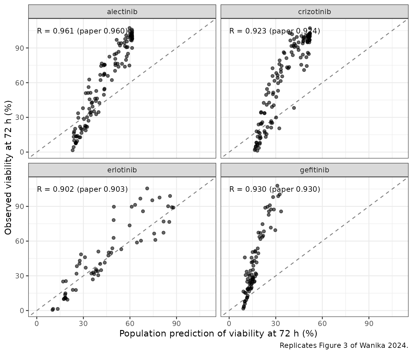
The predictions are deterministic (typical parameters, no random draws), so the correlation is a direct check of the transcribed parameters and structure. The paper’s own ranges are also reproduced: the alectinib predictions sit in a narrow band that never falls below about 20% viability, erlotinib spans almost the full range, and gefitinib stays below about 40% (Results, “Prediction versus observation”).
Concentration-response curves (replicates Figure S1)
Supplementary Figure S1 shows the population-prediction concentration-response curve at 72 h for one reference cell line per drug (H3122 for alectinib and crizotinib, HCC827 for erlotinib, PC9 for gefitinib). Each source study reported its own IC50 and IMAX, so a curve is drawn for every study of that cell line.
ref_cell <- c(alectinib = "H3122", crizotinib = "H3122", erlotinib = "HCC827", gefitinib = "PC9")
grid_conc <- 10^seq(-4, 1.5, length.out = 40)
s1 <- bind_rows(lapply(drugs, function(dr) {
  studies <- curves |>
    filter(drug == dr, cell == ref_cell[[dr]]) |>
    distinct(ref, IC50_VIABILITY, IMAX_VIABILITY)
  g <- studies |>
    tidyr::crossing(conc = grid_conc) |>
    mutate(ID = row_number())
  sim <- solve_typ(mods_typ[[dr]], make_events(g, 72))
  sim |>
    select(ID = id, pred = viability) |>
    left_join(g, by = "ID") |>
    mutate(drug = dr)
}))
#> ℹ omega/sigma items treated as zero: 'etalk_medium_intracellular', 'etalk_intracellular_medium', 'etalvr', 'etalkin', 'etalkout'
#> ℹ omega/sigma items treated as zero: 'etalk_medium_intracellular', 'etalk_intracellular_medium', 'etalvr', 'etalkin', 'etalkout'
#> ℹ omega/sigma items treated as zero: 'etalk_medium_intracellular', 'etalk_intracellular_medium', 'etalvr', 'etalkin', 'etalkout'
#> ℹ omega/sigma items treated as zero: 'etalk_medium_intracellular', 'etalk_intracellular_medium', 'etalvr', 'etalkin', 'etalkout'
s1_obs <- curves |> filter(cell == ref_cell[drug], !is.na(obs))
ggplot(s1, aes(conc, pred, group = interaction(ref, IC50_VIABILITY))) +
  geom_line(linetype = "dashed") +
  geom_point(data = s1_obs, aes(conc, obs, colour = factor(ref)), inherit.aes = FALSE) +
  scale_x_log10() +
  facet_wrap(~ paste0(drug, " (", ref_cell[drug], ")")) +
  labs(
    x = "Medium concentration (umol/L)", y = "Viability at 72 h (%)", colour = "Source study",
    caption = "Replicates supplementary Figure S1 of Wanika 2024 (dashed: population prediction per source study)."
  ) +
  theme_bw()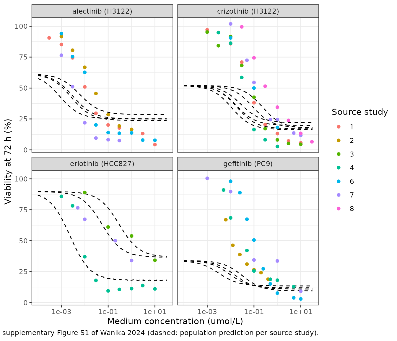
As in the paper’s Figure S1, the population curves start well below 100% at the lowest concentrations, because is below 100% for every fit, and they cover only part of the observed range. The paper attributes this to the population model alone being unable to span the between-study differences, which the random effects absorb (Figure 4).
Variability across curves
Figure 5 of the paper overlays simulations from each curve’s individual (empirical Bayes) parameter estimates, which are not published. As the corresponding check, 100 virtual curves per concentration are drawn from the published between-curve variability for the same reference cell lines, using the IC50 and IMAX of the study with the most curves for that cell line.
rxode2::rxSetSeed(20240311)
n_rep <- 100
vpc <- bind_rows(lapply(drugs, function(dr) {
  obs_cell <- curves |> filter(drug == dr, cell == ref_cell[[dr]])
  main_ref <- names(which.max(table(obs_cell$ref)))
  st <- obs_cell |> filter(ref == main_ref)
  g <- st |>
    distinct(IC50_VIABILITY, IMAX_VIABILITY) |>
    slice(1) |>
    tidyr::crossing(conc = sort(unique(st$conc)), rep = seq_len(n_rep)) |>
    mutate(ID = row_number())
  sim <- rxode2::rxSolve(mods[[dr]], make_events(g, 72), returnType = "data.frame")
  sim |>
    select(ID = id, ipred = viability) |>
    left_join(g, by = "ID") |>
    group_by(conc) |>
    summarise(
      p05 = quantile(ipred, 0.05), p50 = median(ipred), p95 = quantile(ipred, 0.95),
      .groups = "drop"
    ) |>
    mutate(drug = dr, ref = main_ref)
}))
vpc_obs <- curves |>
  semi_join(distinct(vpc, drug, ref), by = c("drug", "ref")) |>
  filter(cell == ref_cell[drug], !is.na(obs))
ggplot(vpc, aes(conc)) +
  geom_ribbon(aes(ymin = p05, ymax = p95), fill = "steelblue", alpha = 0.25) +
  geom_line(aes(y = p50), colour = "steelblue") +
  geom_point(data = vpc_obs, aes(conc, obs)) +
  scale_x_log10() +
  facet_wrap(~ paste0(drug, " (", ref_cell[drug], ")")) +
  labs(
    x = "Medium concentration (umol/L)", y = "Viability at 72 h (%)",
    caption = "Median and 90% interval of 100 simulated curves per concentration; points are the source-study observations."
  ) +
  theme_bw()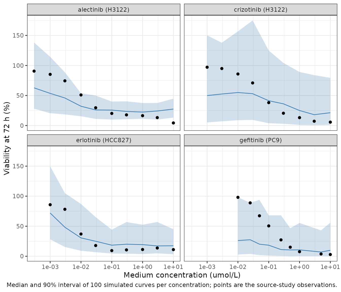
Mechanism check: time course and mass balance
The time course for one H3122 alectinib curve (0.1 umol/L) shows the drug moving from the medium into the cells and the delayed fall in viability. Writing the drug amount per unit initial cell volume as , the model implies : the only change in total drug is the drug carried away with the lost cell volume. The check below integrates the right-hand side on a fine grid and compares it with the solved states.
Note also that is below 100% for every drug (about 51% for alectinib), so the model’s untreated viability also declines from 100% over the 72 h; the published estimates imply this for every fit.
one <- curves |> filter(drug == "alectinib", ID == 6)
tc <- solve_typ(mods_typ$alectinib, make_events(one, seq(0, 72, by = 0.02)))
#> ℹ omega/sigma items treated as zero: 'etalk_medium_intracellular', 'etalk_intracellular_medium', 'etalvr', 'etalkin', 'etalkout'
vr_typ <- exp(mods$alectinib$theta[["lvr"]])
tc <- tc |>
  mutate(
    vc_rel = viability / 100,
    amount_rel = vr_typ * medium + vc_rel * intracellular,
    lost = c(0, cumsum(diff(vc_rel) * (head(intracellular, -1) + tail(intracellular, -1)) / 2))
  )
# Same parameters on both sides: the residual is trapezoidal error only.
stopifnot(
  abs(tc$amount_rel[1] - vr_typ * one$conc) < 1e-8,
  all(abs(tc$amount_rel - tc$amount_rel[1] - tc$lost) < 1e-3 * vr_typ * one$conc)
)
tc |>
  filter(time %in% c(0, 12, 24, 48, 72)) |>
  transmute(
    "Time (h)" = time, "Medium (umol/L)" = signif(medium, 3),
    "Intracellular (umol/L)" = signif(intracellular, 3), "Viability (%)" = signif(viability, 3),
    "Drug remaining (% of dose)" = round(100 * amount_rel / amount_rel[1], 1)
  ) |>
knitr::kable()| Time (h) | Medium (umol/L) | Intracellular (umol/L) | Viability (%) | Drug remaining (% of dose) |
|---|---|---|---|---|
| 0 | 0.10000 | 0.000 | 100.0 | 100.0 |
| 12 | 0.00963 | 0.376 | 78.6 | 82.5 |
| 24 | 0.00779 | 0.386 | 61.9 | 66.8 |
| 48 | 0.00514 | 0.408 | 38.7 | 44.1 |
| 72 | 0.00345 | 0.430 | 24.7 | 29.7 |
tc |>
  select(time, medium, intracellular, viability) |>
  pivot_longer(-time) |>
  ggplot(aes(time, value)) +
  geom_line() +
  facet_wrap(~name, scales = "free_y") +
  labs(x = "Time (h)", y = NULL, caption = "Concentrations in umol/L; viability in %.") +
  theme_bw()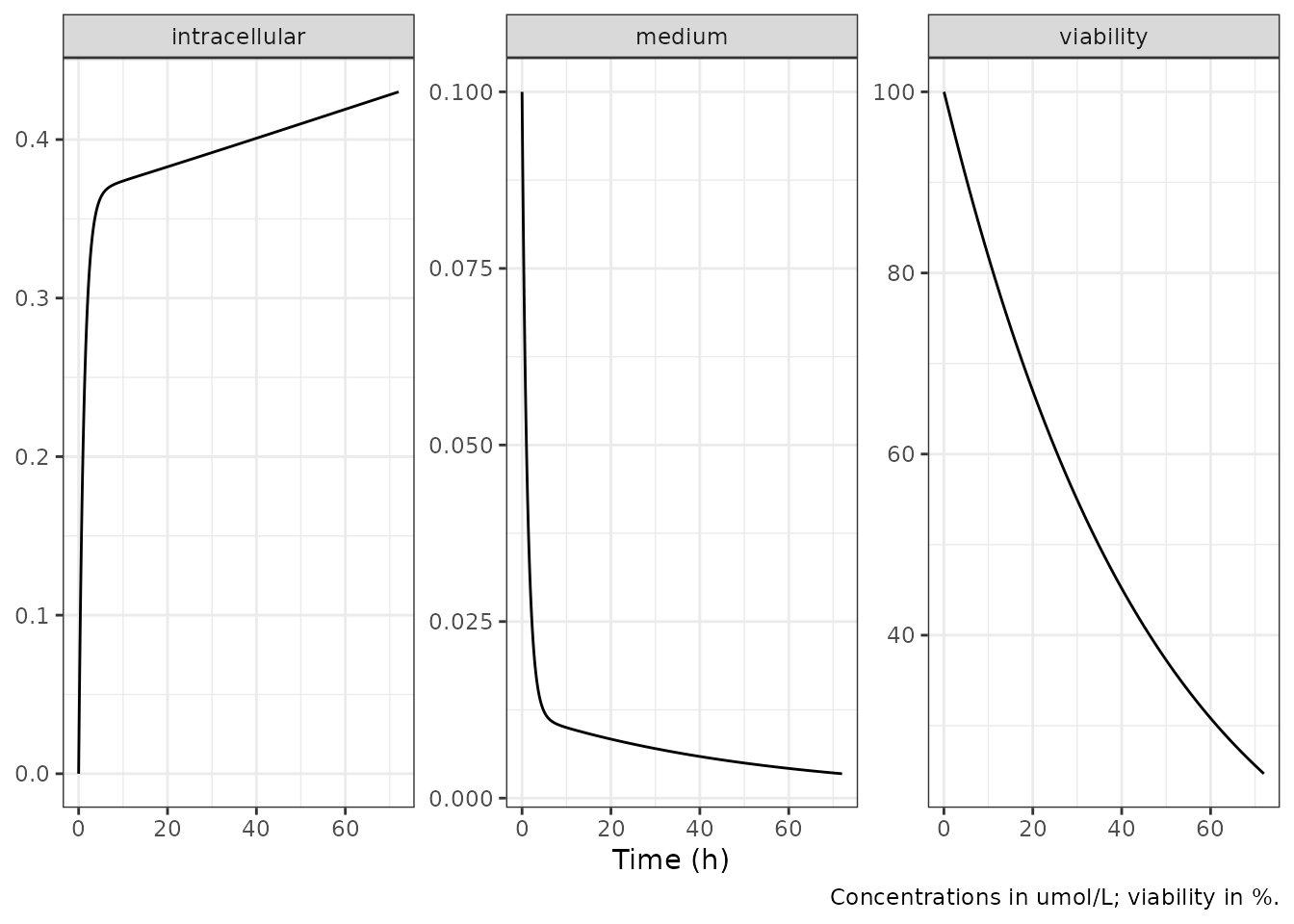
NCA
A non-compartmental analysis is not meaningful for this model: the drug is a single bolus into a closed culture well with no elimination, and the paper reports no exposure metrics. The validation above instead uses the paper’s own prediction-versus-observation correlation (Figure 3) and the drug-balance identity of the structural model.
Assumptions and deviations
-
IMAX is a fraction. Table 1 lists the unit of IMAX
as %, but the values supplied in Tables S1-S4 (0.57-0.99) and Eq 4 use a
fraction;
IMAX_VIABILITYtakes the fraction. - IC50 is the source study’s medium IC50. Eq 4 applies it to the intracellular concentration; the model follows the paper exactly.
-
Residual error magnitudes. Table 2 reports the
constant residual error
aas 16.196 (alectinib), 0.0136 (crizotinib), 0.003 (erlotinib) and 0.737 (gefitinib). On the % viability scale of the data, only the alectinib value is of the size expected from the scatter in Figure 3; the others are reproduced as printed. The residual error does not affect any typical-value or between-curve simulation in this article. - Near-100% shrinkage. Several IIV variances have shrinkage of 99-100% in Table 2 (all five alectinib and gefitinib transfer and volume terms). They are carried as published.
- Supplement transcription. Crizotinib curve ID 29 has only its time-zero record in Table S2, so 128 of the paper’s 129 crizotinib curves have a 72-h observation. Erlotinib curve ID 19 lists IMAX 0.89429 on its time-zero row and 0.88953 on its 72-h row in Table S3; the time-zero value, which governs the 0-72 h dynamics, is used here.
- Figure 5 is not replicated exactly. It uses individual parameter estimates that are not published; the between-curve simulation above is the corresponding population-level check.