Long-acting injectable risperidone: Rykindo and Risperdal Consta (Wang 2024) • nlmixr2lib

Model and source

Wang 2024 developed two population PK models – one for each long-acting injectable (LAI) risperidone formulation – and used them to derive the dosing strategy for switching patients onto RYKINDO. The two models were fitted independently to different (partly overlapping) trial cohorts, so they are packaged as two model files sharing this vignette.

#> ℹ parameter labels from comments will be replaced by 'label()'

Wang_2024_risperidone_rykindo – Population PK model for the risperidone active moiety (risperidone + 9-OH-risperidone) after intramuscular gluteal injection of RYKINDO (LY03004), a biweekly long-acting injectable risperidone formulation, in adults with schizophrenia or schizoaffective disorder (Wang 2024). One-compartment disposition fed by three parallel release pathways out of the injection site: (1) an immediate zero-order release of fraction F2 directly into the central compartment over duration D2, (2) a middle release of fraction F3 = 1 - F1 - F2 delivered as a zero-order input of duration D3 into a second depot beginning ALAG3 after injection and then absorbed first-order with rate K32, and (3) a main first-order release of fraction F1 from the primary depot beginning ALAG1 after injection with absorption rate constant KA. Because the active moiety displays flip-flop kinetics, the elimination rate constant K was set equal to KA, so the apparent central volume is derived as V = CL/KA. Apparent clearance carries a sex effect (females about 18 percent lower) and a between-study effect (0.675-fold in the two US relative-bioavailability trials relative to the single-ascending-dose trial); KA is higher in the multiple-dose trial. The companion RISPERDAL CONSTA model from the same paper is modellib(‘Wang_2024_risperidone_consta’).

#> ℹ parameter labels from comments will be replaced by 'label()'

Wang_2024_risperidone_consta – Population PK model for the risperidone active moiety (risperidone + 9-OH-risperidone) after intramuscular gluteal injection of RISPERDAL CONSTA, the reference biweekly long-acting injectable risperidone formulation, in adults with schizophrenia or schizoaffective disorder (Wang 2024). Same structure as the companion Rykindo model: one-compartment disposition fed by three parallel release pathways out of the injection site, namely an immediate zero-order release of fraction F2 into the central compartment over duration D2, a middle release of fraction F3 = 1 - F1 - F2 entering a second depot as a zero-order input of duration D3 after lag ALAG3 and then absorbed first-order with rate K32, and a main first-order release of fraction F1 beginning ALAG1 = 27 days after injection. The long main-release lag reproduces the well-known 3-week delay that obliges 3 weeks of oral risperidone supplementation when Consta is started. Because the active moiety displays flip-flop kinetics, the elimination rate constant K was set equal to KA, so the apparent central volume is derived as V = CL/KA. Apparent clearance is a single value across trials and sexes; only the main-release absorption rate constant differs between the two trials. The companion Rykindo model is modellib(‘Wang_2024_risperidone_rykindo’).

#> ℹ parameter labels from comments will be replaced by 'label()'

Citation: Wang W, Wang X, Dong Y, Walling DP, Liu P, Liu W, Shi Y, Sun K. Population Pharmacokinetic Analysis to Support and Facilitate Switching from Risperidone Formulations to Rykindo in Patients with Schizophrenia. Neurol Ther. 2024;13(2):355-372. doi:10.1007/s40120-024-00578-w.
Article: https://doi.org/10.1007/s40120-024-00578-w
Supplement (Tables S1-S3, Figures S1-S3): https://doi.org/10.1007/s40120-024-00578-w

Both models describe the active moiety (risperidone + 9-OH-risperidone), which is the pharmacologically relevant species: the two compounds have equivalent activity, so once they are summed the CYP2D6 metabolizer status stops mattering and drops out of the covariate model.

Structure

Both formulations share one structural model (Wang 2024 Figure 2b). A single intramuscular gluteal injection is split three ways at the injection site:

Pathway	Fraction	Input	Onset	Reaches `central` via
Immediate release	`F2`	zero-order, duration `D2`	at injection	directly
Middle release	`F3 = 1 - F1 - F2`	zero-order, duration `D3`	after lag `ALAG3`	`depot2`, then first-order `K32`
Main release	`F1`	first-order, rate `KA`	after lag `ALAG1`	`depot`

Disposition is one-compartment with apparent clearance CL. The initial fit gave an elimination rate constant (0.379 /day) essentially equal to the absorption rate constant (0.322 /day), i.e. flip-flop kinetics, so the authors set K = KA; the apparent central volume is therefore derived as V = CL/KA rather than estimated.

The single structural difference that matters clinically lives entirely in the release parameters: Consta holds ALAG1 = 27 days and puts 75.5% of the dose in the main release, which is the origin of the well-known 3-week lag that obliges 3 weeks of oral risperidone supplementation. Rykindo moves the main release forward to ALAG1 = 13.3 days and redistributes the dose across the three pathways, so it needs only 1 week of oral supplementation.

Population

#> ℹ parameter labels from comments will be replaced by 'label()'

The Rykindo model was fitted to 97 subjects across 3 phase 1 trials (2216 plasma concentration records of risperidone and 9-OH-risperidone (Wang 2024 Results, ‘Population Pharmacokinetic Modeling of Rykindo’).).

Three phase 1 trials in stable adults with schizophrenia or schizoaffective disorder contributed data (Wang 2024 Table 1; 171 patients in total):

Trial	Design	Rykindo	Consta
CT-1S01 (NCT02055287)	single ascending dose, 12.5 / 25 / 37.5 / 50 mg	32 subjects	–
CT-USA-104 (NCT02186769)	parallel single dose, 25 and 50 mg	16 subjects	15 subjects
CT-USA-102 (NCT02091388)	parallel, 25 mg every 2 weeks x 5	54 subjects	54 subjects

Subjects were predominantly male (about 25% female), middle-aged (median 51-55 years) and overweight (median weight 79-90 kg, median BMI 25.4-29.6 kg/m^2). Age, weight, BMI, sex and race were screened as covariates; only sex (on Rykindo clearance) and trial were retained. Race is not reported numerically in the paper. The same information is available programmatically via rxode2::rxode(readModelDb("Wang_2024_risperidone_rykindo"))$population.

Source trace

Every ini() entry carries an in-file comment pointing at its source location. They are collected here for review. All parameter values come from Wang 2024 Table 2 (final model estimates; standard errors from 200 bootstrap replicates because the covariance step failed).

Parameter	Rykindo	Consta	Source
`lcl` (male, CT-1S01 for Rykindo)	186.7 L/day	108.0 L/day	Table 2, rows `CL_male_CT-1S01` / `CL`
`e_sexf_cl`	log(153.4 / 186.7)	not retained	Table 2, row `CL_female_CT-1S01` = 153.4 L/day
`e_studyctusa_cl`	log(0.675)	not retained	Table 2, row `CL ratio for CT-USA-104 and 102 to CT-1S01`
`lka` (main release)	0.288 /day	0.179 /day	Table 2, row `KA_CT-1S01 and CT-USA-104` (footnote: `KA_CT-USA-104` for Consta)
`e_study102_ka`	log(0.380 / 0.288)	log(0.271 / 0.179)	Table 2, row `KA_CT-USA-102`
`ltlag_main` (`ALAG1`)	13.3 day	27.0 day	Table 2, row `ALAG1`
`logitffo` (`F1`)	qlogis(0.430)	qlogis(0.755)	Table 2, row `F1`
`ld2` (`D2`)	0.764 day	0.0467 day	Table 2, row `D2`
`logitfburst` (`F2`)	qlogis(0.148 / (1 - 0.430))	qlogis(0.119 / (1 - 0.755))	Table 2, row `F2`
`ltlag_mid` (`ALAG3`)	3.47 day	0.0417 day	Table 2, row `ALAG3`
`ld3` (`D3`)	2.18 day	23.9 day	Table 2, row `D3`
`lka_mid` (`K32`)	0.118 /day	0.0830 /day	Table 2, row `K32`
`etalcl`	35% CV	34% CV	Table 2, IIV column
`etalka`	27% CV	26% CV	Table 2, IIV column
`etald2`	52% CV	fixed 0	Table 2, IIV column
`etalogitffo`	logit variance 1.3958	fixed 0	Table 2 IIV `F1` = 52% CV (Rykindo); Consta entry uninterpretable, see Errata
`etalogitfburst`	logit variance 0.2605	fixed 0	Table 2 IIV `F2` = 57% CV (Rykindo); Consta entry uninterpretable, see Errata
`etaltlag_main`	fixed 0	fixed 0	Table 2 `ALAG1` IIV `Fix to 0` (Rykindo); Consta entry uninterpretable, see Errata
`addSd`	0.363 ng/mL	0.0546 ng/mL	Table 2, row `add`
`propSd`	26%	32%	Table 2, row `prop`
Structure (three parallel release pathways, `K = KA`)	n/a	n/a	Figure 2b; Results, “Population Pharmacokinetic Modeling of Rykindo”

Release fractions reproduce Table 2

F3 is a derived quantity (F3 = 1 - F1 - F2), so it is a direct check that the logit encoding of the two estimated fractions is correct.

releaseFractions <- function(nm) {
  th <- rxode2::rxode(readModelDb(nm))$theta
  ffo <- plogis(th[["logitffo"]])
  fburst <- (1 - ffo) * plogis(th[["logitfburst"]])
  c(F1 = ffo, F2 = fburst, F3 = 1 - ffo - fburst)
}
fracTable <- rbind(
  Rykindo = releaseFractions("Wang_2024_risperidone_rykindo"),
  Consta  = releaseFractions("Wang_2024_risperidone_consta")
)
#> ℹ parameter labels from comments will be replaced by 'label()'
#> ℹ parameter labels from comments will be replaced by 'label()'
knitr::kable(
  fracTable, digits = 3,
  caption = paste("Release fractions at typical values. Wang 2024 Table 2",
                  "reports F1 = 0.430 / 0.755, F2 = 0.148 / 0.119 and",
                  "F3 = 0.421 / 0.126 for Rykindo / Consta.")
)

Release fractions at typical values. Wang 2024 Table 2 reports F1 = 0.430 / 0.755, F2 = 0.148 / 0.119 and F3 = 0.421 / 0.126 for Rykindo / Consta.
	F1	F2	F3
Rykindo	0.430	0.148	0.422
Consta	0.755	0.119	0.126

Virtual cohort

Original observed data are not publicly available. The simulations below use virtual populations whose sex distribution matches the published trial demographics (Wang 2024 Table 1).

Each intramuscular injection needs three simultaneous dose records – one per release pathway – all carrying the full injected amount; the model’s f() multipliers do the splitting. rxode2 rejects two rate = -2 (modelled duration) records that share a time stamp, so the depot2 record is offset by 1e-4 day (about 9 seconds), which is negligible against a 14-day dosing interval.

set.seed(20240120)

# CT-USA-104 PK sampling schedule (Wang 2024 Table S1), converted to days.
sampleDaysSingle <- c(0, 1 / 24, 3 / 24, 8 / 24, 2, 5, 8, 11, 15, 18,
                      22, 25, 29, 32, 36, 39, 43, 50, 57)

#' Build an event table for one arm.
#'
#' @param n number of subjects (never more than 200 per arm)
#' @param dose injected amount, mg
#' @param covs named list of per-subject covariate vectors (length n)
#' @param obsTimes observation times, days
#' @param nDose number of Q2W injections
#' @param idOffset shifts subject IDs so arms can be bound without colliding
makeArm <- function(n, dose, covs, obsTimes, nDose = 1L, idOffset = 0L,
                    ii = 14) {
  ids <- idOffset + seq_len(n)
  doseTimes <- (seq_len(nDose) - 1L) * ii
  dosing <- lapply(doseTimes, function(tt) {
    bind_rows(
      tibble(id = ids, time = tt,          amt = dose, evid = 1L, cmt = "depot",   rate = 0),
      tibble(id = ids, time = tt,          amt = dose, evid = 1L, cmt = "central", rate = -2),
      tibble(id = ids, time = tt + 1e-4,   amt = dose, evid = 1L, cmt = "depot2",  rate = -2)
    )
  })
  obs <- crossing(id = ids, time = obsTimes) |>
    mutate(amt = 0, evid = 0L, cmt = "central", rate = 0)
  ev <- bind_rows(c(dosing, list(obs)))
  for (nm in names(covs)) ev[[nm]] <- covs[[nm]][match(ev$id, ids)]
  arrange(ev, id, time, desc(evid))
}

nPerArm <- 200L

# Sex mix: Rykindo cohorts were 24.5% female (Table 1); Consta cohorts 26.1%.
rykCovs <- function(n) list(SEXF = rbinom(n, 1, 0.245),
                            STUDY_CT_USA = rep(1L, n),
                            STUDY_CT_USA_102 = rep(0L, n))
conCovs <- function(n) list(STUDY_CT_USA_102 = rep(0L, n))

singleDose <- bind_rows(
  makeArm(nPerArm, 25, rykCovs(nPerArm), sampleDaysSingle, idOffset =   0L) |>
    mutate(treatment = "Rykindo 25 mg", drug = "Rykindo", dose = 25),
  makeArm(nPerArm, 50, rykCovs(nPerArm), sampleDaysSingle, idOffset = 200L) |>
    mutate(treatment = "Rykindo 50 mg", drug = "Rykindo", dose = 50),
  makeArm(nPerArm, 25, conCovs(nPerArm), sampleDaysSingle, idOffset = 400L) |>
    mutate(treatment = "Consta 25 mg",  drug = "Consta",  dose = 25),
  makeArm(nPerArm, 50, conCovs(nPerArm), sampleDaysSingle, idOffset = 600L) |>
    mutate(treatment = "Consta 50 mg",  drug = "Consta",  dose = 50)
)
stopifnot(!anyDuplicated(unique(singleDose[, c("id", "time", "evid")])))

Simulation

modRyk <- readModelDb("Wang_2024_risperidone_rykindo")
modCon <- readModelDb("Wang_2024_risperidone_consta")

simArm <- function(mod, ev, keepCols) {
  rxode2::rxSolve(mod, events = as.data.frame(ev), keep = keepCols,
                  addDosing = FALSE) |>
    as.data.frame()
}

simSingle <- bind_rows(
  simArm(modRyk, filter(singleDose, drug == "Rykindo"),
         c("treatment", "drug", "dose", "SEXF")),
  simArm(modCon, filter(singleDose, drug == "Consta"),
         c("treatment", "drug", "dose"))
) |>
  mutate(Cc = pmax(Cc, 0), sim = pmax(sim, 0), CcNorm = Cc / dose)
#> ℹ parameter labels from comments will be replaced by 'label()'
#> ℹ omega/sigma items treated as zero: 'etaltlag_main', 'etaltlag_mid', 'etald3', 'etalka_mid'
#> ℹ parameter labels from comments will be replaced by 'label()'
#> ℹ omega/sigma items treated as zero: 'etald2', 'etalogitffo', 'etalogitfburst', 'etaltlag_main', 'etaltlag_mid', 'etald3', 'etalka_mid'

Typical-value (no between-subject variability) profiles are used to replicate the paper’s descriptive statements about release timing.

typicalTimes <- seq(0, 57, by = 0.05)
typicalArm <- function(mod, dose, covs) {
  ev <- makeArm(1L, dose, lapply(covs, function(x) x), typicalTimes)
  rxode2::rxSolve(rxode2::zeroRe(mod), events = as.data.frame(ev),
                  addDosing = FALSE) |>
    as.data.frame()
}
simTypical <- bind_rows(
  typicalArm(modRyk, 25, list(SEXF = 0L, STUDY_CT_USA = 1L, STUDY_CT_USA_102 = 0L)) |>
    mutate(treatment = "Rykindo 25 mg", dose = 25),
  typicalArm(modRyk, 50, list(SEXF = 0L, STUDY_CT_USA = 1L, STUDY_CT_USA_102 = 0L)) |>
    mutate(treatment = "Rykindo 50 mg", dose = 50),
  typicalArm(modCon, 25, list(STUDY_CT_USA_102 = 0L)) |>
    mutate(treatment = "Consta 25 mg", dose = 25),
  typicalArm(modCon, 50, list(STUDY_CT_USA_102 = 0L)) |>
    mutate(treatment = "Consta 50 mg", dose = 50)
)
#> ℹ parameter labels from comments will be replaced by 'label()'
#> ℹ omega/sigma items treated as zero: 'etalcl', 'etalka', 'etald2', 'etalogitffo', 'etalogitfburst', 'etaltlag_main', 'etaltlag_mid', 'etald3', 'etalka_mid'
#> ℹ parameter labels from comments will be replaced by 'label()'
#> ℹ omega/sigma items treated as zero: 'etalcl', 'etalka', 'etald2', 'etalogitffo', 'etalogitfburst', 'etaltlag_main', 'etaltlag_mid', 'etald3', 'etalka_mid'
#> ℹ parameter labels from comments will be replaced by 'label()'
#> ℹ omega/sigma items treated as zero: 'etalcl', 'etalka', 'etald2', 'etalogitffo', 'etalogitfburst', 'etaltlag_main', 'etaltlag_mid', 'etald3', 'etalka_mid'
#> ℹ parameter labels from comments will be replaced by 'label()'
#> ℹ omega/sigma items treated as zero: 'etalcl', 'etalka', 'etald2', 'etalogitffo', 'etalogitfburst', 'etaltlag_main', 'etaltlag_mid', 'etald3', 'etalka_mid'

Replicate published figures

Figure 1a – single-dose profiles of Rykindo versus Consta

# Replicates Figure 1a of Wang 2024: plasma active moiety after a single IM
# injection of Rykindo or Consta at 25 and 50 mg.
ggplot(simTypical, aes(time, Cc, colour = treatment, linetype = treatment)) +
  geom_line(linewidth = 0.8) +
  scale_x_continuous(breaks = seq(0, 56, by = 7)) +
  labs(x = "Time after dose (day)", y = "Active moiety (ng/mL)",
       colour = NULL, linetype = NULL,
       title = "Figure 1a -- single IM injection, typical-value profiles",
       caption = "Replicates Figure 1a of Wang 2024.") +
  theme(legend.position = "bottom")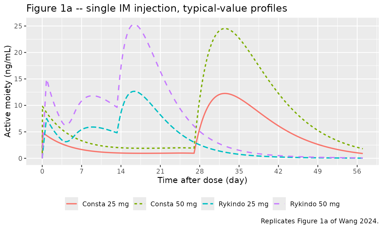

The model reproduces the paper’s central descriptive claim: Rykindo rises immediately and peaks around day 15-17, whereas Consta stays at a low near-flat plateau for about 3 weeks before its main release drives a peak around day 32-34.

simTypical |>
  group_by(treatment) |>
  summarise(`Tmax (day)` = round(time[which.max(Cc)], 1),
            `Cmax (ng/mL)` = round(max(Cc), 2), .groups = "drop") |>
  knitr::kable(caption = paste(
    "Typical-value Tmax. Wang 2024 Results report observed Tmax of days 14-17",
    "for Rykindo and days 32-34 (median) for Consta in trial CT-USA-104."))

Typical-value Tmax. Wang 2024 Results report observed Tmax of days 14-17 for Rykindo and days 32-34 (median) for Consta in trial CT-USA-104.
treatment	Tmax (day)	Cmax (ng/mL)
Consta 25 mg	32.5	12.26
Consta 50 mg	32.5	24.52
Rykindo 25 mg	16.4	12.65
Rykindo 50 mg	16.4	25.31

Figures 3a and 4a – visual predictive checks

Wang 2024 plots dose-normalised concentrations. Both published panels are the 25 mg single-dose arm, so the comparison below is restricted to that arm. The dashed percentile curves in the published figures are the model’s own 2.5th / 50th / 97.5th prediction percentiles.

# Replicates Figures 3a (Rykindo) and 4a (Consta) of Wang 2024.
vpc <- simSingle |>
  filter(dose == 25) |>
  mutate(dvNorm = sim / dose) |>
  group_by(drug, time) |>
  summarise(Q025 = quantile(dvNorm, 0.025), Q50 = quantile(dvNorm, 0.5),
            Q975 = quantile(dvNorm, 0.975), .groups = "drop")

ggplot(vpc, aes(time, Q50)) +
  geom_ribbon(aes(ymin = Q025, ymax = Q975), alpha = 0.25, fill = "steelblue") +
  geom_line(linewidth = 0.8) +
  facet_wrap(~drug) +
  scale_x_continuous(breaks = seq(0, 56, by = 14)) +
  labs(x = "Time after dose (day)",
       y = "Active moiety normalised by dose (ng/mL/mg)",
       title = "Figures 3a / 4a -- single 25 mg dose, dose-normalised",
       caption = paste("Replicates Figures 3a (Rykindo) and 4a (Consta) of",
                       "Wang 2024. Ribbon = 2.5th-97.5th percentile."))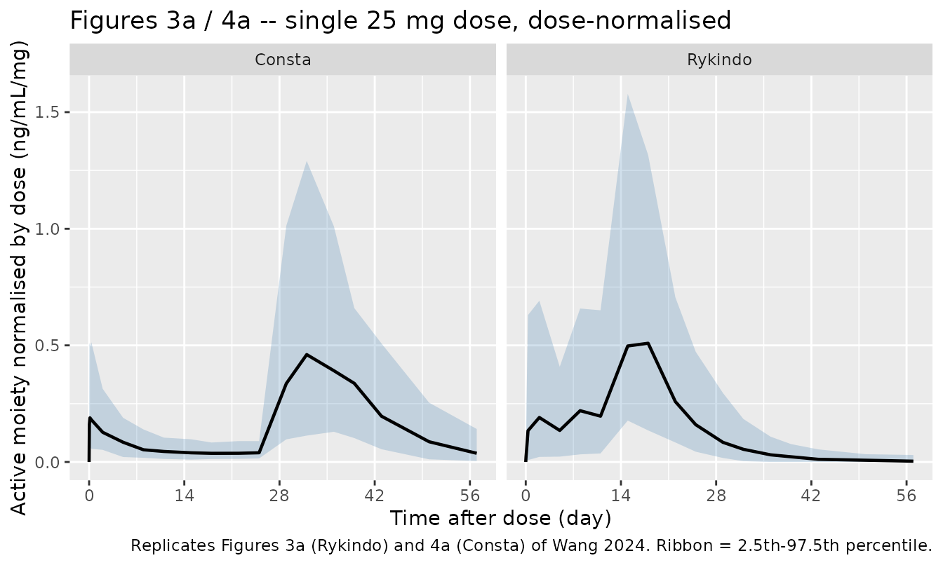

The peak of each published percentile band can be read off the source figures and compared numerically.

vpcPeak <- vpc |>
  group_by(drug) |>
  slice_max(Q50, n = 1) |>
  ungroup() |>
  transmute(drug, `Peak time (day)` = time,
            `2.5th` = Q025, Median = Q50, `97.5th` = Q975)

published <- tibble::tribble(
  ~drug,     ~`Peak time (day)`, ~`2.5th`, ~Median, ~`97.5th`,
  "Rykindo",  17,                 0.17,     0.48,    1.02,
  "Consta",   31,                 0.27,     0.58,    1.39
)

bind_rows(mutate(vpcPeak, source = "simulated"),
          mutate(published, source = "Wang 2024 Fig 3a / 4a (read off plot)")) |>
  relocate(source) |>
  arrange(drug, source) |>
  knitr::kable(digits = 2, caption = paste(
    "Dose-normalised prediction percentiles at their peak. Published values",
    "were read off the published figures and are approximate."))

Dose-normalised prediction percentiles at their peak. Published values were read off the published figures and are approximate.
source	drug	Peak time (day)	2.5th	Median	97.5th
Wang 2024 Fig 3a / 4a (read off plot)	Consta	31	0.27	0.58	1.39
simulated	Consta	32	0.11	0.46	1.29
Wang 2024 Fig 3a / 4a (read off plot)	Rykindo	17	0.17	0.48	1.02
simulated	Rykindo	18	0.14	0.51	1.32

PKNCA validation

Wang 2024 reports observed single-dose NCA from trial CT-USA-104 (Results, “PK of Rykindo from the Phase I Clinical Trials”): geometric-mean Cmax and AUC0-t, with sampling truncated at day 57. The simulated NCA is computed on exactly that sampling schedule so the comparison is like for like.

simNca <- simSingle |>
  filter(!is.na(sim)) |>
  transmute(id, time, Cc = sim, treatment)

# Guarantee a time = 0 record per subject (pre-dose Cc = 0 for an IM depot).
simNca <- bind_rows(
  simNca,
  simNca |> distinct(id, treatment) |> mutate(time = 0, Cc = 0)
) |>
  distinct(id, treatment, time, .keep_all = TRUE) |>
  arrange(id, treatment, time)

concObj <- PKNCA::PKNCAconc(simNca, Cc ~ time | treatment + id)

doseDf <- singleDose |>
  filter(evid == 1L, cmt == "depot") |>
  transmute(id, time, amt, treatment)
doseObj <- PKNCA::PKNCAdose(doseDf, amt ~ time | treatment + id)

intervals <- data.frame(start = 0, end = 57,
                        cmax = TRUE, tmax = TRUE, auclast = TRUE)

ncaRes <- PKNCA::pk.nca(PKNCA::PKNCAdata(concObj, doseObj, intervals = intervals))

publishedNca <- tibble::tribble(
  ~treatment,      ~cmax, ~tmax, ~auclast,
  "Rykindo 25 mg",  18.5,  15.5,   227,
  "Rykindo 50 mg",  30.0,  15.5,   399,
  "Consta 25 mg",   17.6,  33.0,   193,
  "Consta 50 mg",   36.0,  33.0,   490
)

cmp <- nlmixr2lib::ncaComparisonTable(
  simulated = ncaRes,
  reference = publishedNca,
  by = "treatment",
  units = c(cmax = "ng/mL", tmax = "day", auclast = "day*ng/mL"),
  tolerance_pct = 20
)

knitr::kable(cmp, caption = paste(
  "Simulated versus published single-dose NCA (trial CT-USA-104,",
  "sampling truncated at day 57). * differs from the published value by",
  "more than 20%."), align = c("l", "l", "r", "r"))

Simulated versus published single-dose NCA (trial CT-USA-104, sampling truncated at day 57). * differs from the published value by more than 20%.
NCA parameter	treatment	Reference	Simulated	% diff
Cmax (ng/mL)	Rykindo 25 mg	18.5	15.3	-17.5%
Cmax (ng/mL)	Rykindo 50 mg	30	29.5	-1.7%
Cmax (ng/mL)	Consta 25 mg	17.6	14	-20.6%*
Cmax (ng/mL)	Consta 50 mg	36	28.1	-21.9%*
Tmax (day)	Rykindo 25 mg	15.5	15	-3.2%
Tmax (day)	Rykindo 50 mg	15.5	15	-3.2%
Tmax (day)	Consta 25 mg	33	32	-3.0%
Tmax (day)	Consta 50 mg	33	32	-3.0%
AUClast (day*ng/mL)	Rykindo 25 mg	227	220	-3.0%
AUClast (day*ng/mL)	Rykindo 50 mg	399	416	+4.2%
AUClast (day*ng/mL)	Consta 25 mg	193	231	+19.7%
AUClast (day*ng/mL)	Consta 50 mg	490	461	-6.0%

Tmax agrees to within a day in every arm, and AUC0-t agrees to within about 20% (and to within 5% for both Rykindo arms). Cmax is systematically under-predicted, most markedly for Consta. Two effects drive this and neither is a transcription problem:

The published Cmax is the geometric mean of each subject’s own maximum observed concentration. Individual peaks are sharper than a population mean profile and occur at different times, so this statistic always sits above the peak of the mean profile.
For Consta the model carries between-subject variability only on CL and KA (the release-parameter IIVs reported by the paper are uninterpretable – see Errata below), so the simulated spread of individual peak heights is narrower than the real one and the geometric mean of individual Cmax is correspondingly lower. Rykindo, which retains its release-parameter IIV, is the closer of the two.

The paper’s own visual predictive checks are the cleaner comparison for the peak, because they are percentiles of the model’s predictions rather than a statistic on individual maxima – and there the simulated median peak matches (previous section).

Steady-state exposure comparison (Table S2)

The paper simulated 1000 virtual subjects per arm receiving 25 mg every 2 weeks and compared steady-state exposure over the interval after the sixth injection (day 70 to day 84). The cohort here is capped at 200 per arm.

Seven Q2W injections of a formulation whose middle release runs as a 23.9-day zero-order input (Consta D3) means many overlapping infusions, which makes the solve cost grow steeply with the observation grid. The grid below is therefore coarse outside the steady-state window and finer inside it; against a 0.05-day reference grid this reproduces Cmax,ss and Cmin,ss to within 0.6% and AUCtau,ss to within 0.4%. The cohort is 100 per arm for the same reason.

nSteadyState <- 100L
ssTimes <- sort(unique(c(seq(0, 98, by = 0.5), seq(70, 84, by = 0.25))))
ssRyk <- makeArm(nSteadyState, 25,
                 list(SEXF = rbinom(nSteadyState, 1, 0.245),
                      STUDY_CT_USA = rep(1L, nSteadyState),
                      STUDY_CT_USA_102 = rep(1L, nSteadyState)),
                 ssTimes, nDose = 7L, idOffset = 0L)
ssCon <- makeArm(nSteadyState, 25,
                 list(STUDY_CT_USA_102 = rep(1L, nSteadyState)),
                 ssTimes, nDose = 7L, idOffset = 1000L)

ssSim <- bind_rows(
  simArm(modRyk, ssRyk, character()) |> mutate(drug = "Rykindo"),
  simArm(modCon, ssCon, character()) |> mutate(drug = "Consta")
) |>
  mutate(Cc = pmax(Cc, 0))
#> ℹ omega/sigma items treated as zero: 'etaltlag_main', 'etaltlag_mid', 'etald3', 'etalka_mid'
#> ℹ omega/sigma items treated as zero: 'etald2', 'etalogitffo', 'etalogitfburst', 'etaltlag_main', 'etaltlag_mid', 'etald3', 'etalka_mid'

ssStats <- ssSim |>
  filter(time >= 70, time <= 84) |>
  group_by(drug, id) |>
  arrange(time, .by_group = TRUE) |>
  summarise(
    cmaxss = max(Cc), cminss = min(Cc),
    aucss = sum(diff(time) * (head(Cc, -1) + tail(Cc, -1)) / 2),
    .groups = "drop"
  ) |>
  mutate(cavess = aucss / 14,
         ptf = 100 * (cmaxss - cminss) / cavess)

geomean <- function(x) exp(mean(log(x[x > 0])))
ssRatio <- ssStats |>
  group_by(drug) |>
  summarise(across(c(cmaxss, aucss, cminss, ptf), geomean), .groups = "drop")

ratioRow <- function(par) {
  100 * ssRatio[[par]][ssRatio$drug == "Rykindo"] /
    ssRatio[[par]][ssRatio$drug == "Consta"]
}

tibble::tibble(
  Parameter = c("Cmax,ss", "AUCtau,ss", "Cmin,ss", "PTF%"),
  `Simulated ratio % (Rykindo/Consta)` =
    round(c(ratioRow("cmaxss"), ratioRow("aucss"),
            ratioRow("cminss"), ratioRow("ptf")), 2),
  `Wang 2024 Table S2 ratio %` = c(93.02, 94.43, 121.75, 93.1),
  `Table S2 90% CI` = c("90.62-95.49", "92.00-96.92", "115.91-127.88", "-")
) |>
  knitr::kable(caption = paste(
    "Steady-state exposure of the active moiety, Rykindo relative to Consta",
    "at 25 mg every 2 weeks, over the interval after the sixth injection",
    "(day 70-84). Reference values from Wang 2024 supplementary Table S2."))

Steady-state exposure of the active moiety, Rykindo relative to Consta at 25 mg every 2 weeks, over the interval after the sixth injection (day 70-84). Reference values from Wang 2024 supplementary Table S2.
Parameter	Simulated ratio % (Rykindo/Consta)	Wang 2024 Table S2 ratio %	Table S2 90% CI
Cmax,ss	98.48	93.02	90.62-95.49
AUCtau,ss	85.54	94.43	92.00-96.92
Cmin,ss	100.37	121.75	115.91-127.88
PTF%	112.95	93.10	-

ssSim |>
  group_by(drug, time) |>
  summarise(Q05 = quantile(Cc, 0.05), Q50 = quantile(Cc, 0.5),
            Q95 = quantile(Cc, 0.95), .groups = "drop") |>
  ggplot(aes(time, Q50, colour = drug, fill = drug)) +
  geom_ribbon(aes(ymin = Q05, ymax = Q95), alpha = 0.2, colour = NA) +
  geom_line(linewidth = 0.8) +
  scale_x_continuous(breaks = seq(0, 98, by = 14)) +
  labs(x = "Time (day)", y = "Active moiety (ng/mL)", colour = NULL, fill = NULL,
       title = "25 mg every 2 weeks, seven injections",
       caption = paste("Companion to Wang 2024 Figure 5. Ribbon = 5th-95th",
                       "percentile; line = median.")) +
  theme(legend.position = "bottom")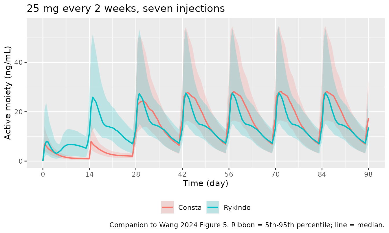

The simulation reproduces the paper’s headline finding that Rykindo reaches steady state roughly two weeks earlier than Consta while delivering comparable steady-state exposure. Cmax,ss lands close to the published ratio. The other three rows deserve comment rather than a claim of agreement:

AUCtau,ss (85.5% simulated versus 94.43% published). Because both formulations are linear and fully absorbed, this ratio is exactly the clearance ratio CL_Consta / CL_Rykindo, with no dependence on the release parameters. Wang 2024 does not describe the virtual population’s covariate distribution, and the ratio is entirely determined by its sex mix: 108.0 / 126.0 = 85.7% for an all-male cohort, 108.0 / 103.5 = 104.3% for an all-female cohort, and 108.0 / sqrt(126.0 * 103.5) = 94.6% for a sex-balanced one. The cohort here uses the trial-observed 24.5% female split, which lands near the male end. The published 94.43% therefore implies the authors simulated a roughly sex-balanced population. This is recorded as an inference about the source, not applied as a calibration.
Cmin,ss (100.4% simulated versus 121.75% published) and PTF (113.0% versus 93.1%). Both say the same thing: relative to Consta, the simulated Rykindo profile troughs lower and fluctuates more than the published one. PTF is a within-subject normalised quantity, so unlike AUC it is not sensitive to the sex mix – it is the same 113% for an all-male and an all-female cohort. The discrepancy instead traces to the Consta model carrying between-subject variability only on CL and KA: with its release-parameter IIV suppressed (see Errata), individual Consta profiles are flatter than the real ones, which depresses Consta’s own PTF and raises the Rykindo-to-Consta ratio. It is the same root cause as the Consta Cmax shortfall in the NCA table above, and it is the main quantitative limitation of this extraction.

Assumptions and deviations

Release fractions are carried on a logit scale with a stick-breaking split. The paper estimates F1 and F2 and derives F3 = 1 - F1 - F2, but does not state the transformation used. Encoding both as plain log-normal random effects with the published CVs (52% and 57% for Rykindo) drives F1 + F2 > 1 – and therefore a negative middle-release fraction – in about 10% of simulated subjects. The packaged models instead use F1 = expit(logitffo + eta) and F2 = (1 - F1) * expit(logitfburst + eta), which guarantees F3 >= 0 for every subject and reproduces the published point estimates exactly at eta = 0 (verified in the “Release fractions” table above). The logit-scale IIV variances (1.3958 and 0.2605) were chosen by moment matching so the simulated coefficient of variation of F1 and F2 equals the published 52% and 57%. logitfburst is therefore stated relative to the non-main-release remainder: qlogis(0.148 / (1 - 0.430)) for Rykindo and qlogis(0.119 / (1 - 0.755)) for Consta, with the paper’s own F1 and F2 values visible verbatim in the expression.

Three Consta IIV entries are set to fixed(0) because the published values carry no interpretable scale. In Wang 2024 Table 2, every IIV entry is reported as a percentage (27%, 35%, 52%, …) except three in the Consta column: F2 = 0.67, ALAG1 = 0.87 and F1 = 0.57. Each candidate reading was tested by simulation against the paper’s own Consta visual predictive check (Figure 4a), which shows a sharp, tightly time-aligned peak at about day 31 with percentile ratios of roughly 2.4 (97.5th / median) and 2.2 (median / 2.5th). The diagnostic below was run separately on the Consta 25 mg single-dose arm (2000 subjects, matching the design of Figure 4a) so that the readings are not confounded by Monte Carlo noise; values are dose-normalised concentrations (ng/mL/mg) at the peak of the median curve:

Reading of `0.67 / 0.87 / 0.57`	Peak day	2.5th	Median	97.5th
Published Figure 4a (read off plot)	~31	0.27	0.58	1.39
CV% (67% / 87% / 57% CV, log-normal)	29	0.00	0.15	0.84
log-scale variance `omega^2`	26	0.00	0.15	0.74
log-scale standard deviation `omega`	26	0.00	0.14	0.77
all three fixed to 0 (packaged)	32	0.16	0.48	1.10

Any log-scale reading of the 0.87 entry implies so much variability on a 27-day lag time that roughly 40% of subjects would not yet have started their main release at day 31; the peak collapses and the published figure could not have been produced. Setting the three to zero reproduces Figure 4a closely. The standing convention for an IIV that cannot be interpreted is to fix it at zero and document, rather than to invent a scale. A user who wants the variability back should note that reading the two fraction entries as logit-scale variances (etalogitffo ~ 0.57, etalogitfburst ~ 0.67) is the only interpretation not refuted by Figure 4a; the ALAG1 entry has no surviving log-scale reading at all. The consequence is visible in the NCA table above, where the simulated Consta Cmax is the furthest below its published value.

V = CL/KA follows the paper’s flip-flop simplification, so it is trial-dependent. Wang 2024 sets the elimination rate constant K equal to the absorption rate constant KA, and KA itself is trial-dependent. The apparent central volume therefore also shifts with STUDY_CT_USA_102. This is a faithful consequence of the paper’s stated simplification, not an added assumption; the resulting typical-value peak (0.49 ng/mL/mg dose-normalised for Rykindo) matches the median of the paper’s own VPC.
Text-versus-table conflict on the clearance ratio, resolved in favour of the table. Wang 2024 Table 2 labels the 0.675 clearance ratio as applying to “CT-USA-104 and 102”, while the Results text describes the reduced clearance as belonging to “the multiple-dose study” (CT-USA-102 alone). The table definition is encoded. It is also the reading the data support: with the ratio applied, the simulated CT-USA-104 AUC0-t is 220 and 416 day*ng/mL at 25 and 50 mg against published values of 227 and 399 (NCA table above); without it, clearance would be 1/0.675 = 1.48-fold higher and the predictions would fall to roughly two thirds of those values, far below the observed exposures.
Sex effect taken from Table 2 rather than the Results text. Table 2 gives 186.7 L/day (male) and 153.4 L/day (female), a ratio of 0.822 (17.8% lower in females). The Results text describes it as “about 15% lower”. The final-model table estimates are used.
The paper’s virtual population is not described. Wang 2024 states only that 1000 virtual subjects per arm were simulated, without giving the covariate distribution. The cohorts here use the trial-observed sex split (24.5% female). Note that a sex-balanced (50/50) virtual population reproduces the published AUCtau,ss ratio of 94.43% almost exactly, because that ratio depends only on the clearance contrast: 108.0 / sqrt(126.0 * 103.5) = 94.6%. This is recorded as an observation about the source, not applied as a calibration.
Steady-state scenario uses the CT-USA-102 absorption parameters. The paper does not say which trial’s KA was used for the model-based simulations. The multiple-dose trial parameters are used here because the simulated scenario is chronic Q2W dosing, and because they reproduce the published Cmin,ss and PTF ratios substantially better than the single-dose parameters do.
Cohort size and Monte Carlo noise. The paper used 1000 subjects per arm; the library cap is 200, and the steady-state arms use 100 to keep the render inside its time budget (see the note above that chunk). With between-subject CVs of 26-52%, the geometric-mean ratios in the Table S2 comparison carry a Monte Carlo standard error of a few percent, so small deviations from the published point estimates are expected even where the model is exact.
Race and ethnicity are not reported in Wang 2024, so no race distribution is simulated. Race was screened as a covariate and not retained.
Cohort-size accounting in the source. Wang 2024 Table 1 lists 102 Rykindo and 69 Consta subjects, while the Results text states that 97 and 66 subjects contributed the analysed concentration records. The difference is not explained in the paper; the population metadata records the Results-text counts and notes the discrepancy.
Supplementary Figures S1-S3 are diagnostic plots (goodness-of-fit and additional switching scenarios) and are not replicated here; the parameter values they support are all in Table 2.