Model and source
- Citation: Cheng X, Zhao Y, Gu H, Zhao L, Zang Y, Wang X, Wu R. The first study in pediatric: Population pharmacokinetics of sirolimus and its application in Chinese children with immune cytopenia. Int J Immunopathol Pharmacol. 2020;34:2058738420934936. doi:10.1177/2058738420934936
- Description: One-compartment population PK model with first-order absorption and elimination for oral sirolimus in Chinese children with refractory immune cytopenia, developed from routine steady-state therapeutic-drug-monitoring trough concentrations (Cheng 2020). Apparent clearance scales with body weight (power exponent 0.50, normalized to the 28.5 kg cohort median) and total bilirubin (power exponent -0.32, normalized to the 11.29 umol/L cohort median); apparent volume carries no covariate. The absorption rate constant was fixed at 0.7521 per hour from the literature because only trough samples were available. Inter-individual variability is exponential on CL/F and V/F and the residual error is proportional.
- Article: https://doi.org/10.1177/2058738420934936 (open access, PMC7388097)
Cheng and colleagues fit a one-compartment model with first-order absorption to 107 routine therapeutic-drug-monitoring (TDM) trough concentrations from 27 Chinese children with refractory immune cytopenia who took oral sirolimus. The analysis used Phoenix NLME 1.3. Of 19 screened covariates, body weight and total bilirubin were retained, both on apparent clearance. The paper’s practical output is Table 4, a table of initial daily doses by body weight and total bilirubin.
Population
The single-centre pilot study at Beijing Children’s Hospital ran from January 2016 to December 2017 (Cheng 2020 Table 1). The 27 children (18 male, 9 female) were 8.16 +/- 3.60 years old (range 1-15) and weighed 27.03 +/- 10.87 kg (range 7-43; median 28.50 kg). Mean total bilirubin was 12.13 +/- 7.35 umol/L (median 11.29 umol/L). Sirolimus gelatin capsules were given orally once daily. The starting dose was 1.5 mg/m^2, and later doses were titrated by TDM to a trough of 5-15 ng/mL. Every concentration is a steady-state trough drawn 0.5 h before the next dose, at least 7 days after the first dose. Whole blood was assayed by fluorescence polarization immunoassay (Abbott TDx/FLx).
The same information is available programmatically via
readModelDb("Cheng_2020_sirolimus")()$population.
Source trace
| Element | Value | Source |
|---|---|---|
| Structure: one compartment, first-order absorption and elimination | – | Methods, ‘PPK analysis’; Results |
lcl (CL/F at 28.5 kg, TBIL 11.29 umol/L) |
5.63 L/h | Table 3; final-model equation (Results) |
lvc (V/F) |
144.16 L | Table 3 |
lka (Ka, held constant) |
0.7521 1/h | Methods, ‘PPK analysis’ (Table 3 prints 0.75, RSE 0) |
e_tbili_cl |
-0.32 | Table 3 ‘f CL-TBIL’; final-model equation |
e_wt_cl |
0.50 | Table 3 ‘f CL-WT’; final-model equation |
| Reference total bilirubin | 11.29 umol/L | Results: ‘11.29 is median TBIL’ |
| Reference body weight | 28.50 kg | Results: ‘The median weight of children was 28.50 kg’ |
etalcl |
0.0353 (log-scale variance) | Abstract: IIV of CL/F 3.53% (see below) |
etalvc |
0.0727 (log-scale variance) | Abstract: IIV of V/F 7.27% (see below) |
propSd |
0.2245 | Abstract: proportional error 22.45%; Table 3 Sigma 0.22 |
| No covariate on V/F | – | Results: ‘V was by no co-variants influenced’ |
The final-model equation printed in Results is
CL (L/h) = 5.63 x (TBIL / 11.29)^-0.32 x (WT / 28.50)^0.5 x exp(eta_CL).
Scale of the inter-individual variability
Table 3 has no omega rows. The only report of the between-subject variability is the abstract: “Inter-individual variabilities for CL/F and V/F were 3.53% and 7.27%, respectively. The intra-individual variability of proportional error model was 22.45%.” Two readings are possible:
-
Omega diagonal times 100 (used). Phoenix NLME
prints the Omega matrix as log-scale variances and the residual term as
a standard deviation (
stdev0). Table 3 gives the residual term as 0.22, and the abstract turns it into “22.45%” by multiplying the printed estimate by 100. Applying the same convention to the omegas gives omega^2 = 0.0353 and 0.0727, which are apparent CVs of about 19% and 27%. - Literal CVs. omega^2 = log(1 + CV^2) = 0.00125 and 0.00527, which are apparent CVs of 3.5% and 7.3%.
No other result in the paper separates the two readings: there is no RSE, no shrinkage and no published prediction interval. The model uses the first reading because it treats the omegas and the residual term the same way. This only affects the stochastic spread in the simulations below. The typical-value checks do not depend on it.
omega_pct <- c(CL = 3.53, V = 7.27)
data.frame(
  parameter = names(omega_pct),
  omega2_used = omega_pct / 100,
  apparent_cv_used_pct = 100 * sqrt(exp(omega_pct / 100) - 1),
  omega2_literal_cv = log(1 + (omega_pct / 100)^2)
) |>
knitr::kable(digits = 5)| parameter | omega2_used | apparent_cv_used_pct | omega2_literal_cv | |
|---|---|---|---|---|
| CL | CL | 0.0353 | 18.95533 | 0.00125 |
| V | V | 0.0727 | 27.46049 | 0.00527 |
Virtual cohort
Table 4 splits patients into four body-weight bands (5-15, 15-25, 25-35 and 35-45 kg) and two total-bilirubin bands (3.42-20.50 and > 20.50 umol/L). It gives a daily initial dose for each of the eight cells. Each cell below has 200 virtual children, with body weight drawn uniformly within the band. Total bilirubin is drawn uniformly over 3.42-20.50 umol/L in the normal band and over 20.50-40 umol/L in the high band. The paper gives no upper bound for the high band, so 40 umol/L is an assumption.
mod <- readModelDb("Cheng_2020_sirolimus")
ui <- rxode2::rxode(mod)
#> ℹ parameter labels from comments will be replaced by 'label()'
theta <- ui$theta

tab4 <- tibble::tribble(
  ~wt_lo, ~wt_hi, ~tbili_band, ~dose_mg,
  5, 15, "normal", 0.75,
  15, 25, "normal", 1.5,
  25, 35, "normal", 1.75,
  35, 45, "normal", 2.0,
  5, 15, "high", 0.5,
  15, 25, "high", 0.75,
  25, 35, "high", 1.0,
  35, 45, "high", 1.5
) |>
  mutate(
    cell = sprintf("WT %g-%g kg, TBIL %s", wt_lo, wt_hi, tbili_band),
    cell_id = row_number()
  )

n_per_cell <- 200
tau <- 24
n_dose <- 56
t_end <- n_dose * tau

rxode2::rxSetSeed(20200701)
subj <- tab4[rep(seq_len(nrow(tab4)), each = n_per_cell), ] |>
  mutate(
    id = row_number(),
    WT = runif(n(), wt_lo, wt_hi),
    TBILI = ifelse(tbili_band == "normal", runif(n(), 3.42, 20.5), runif(n(), 20.5, 40))
  )
stopifnot(!anyDuplicated(subj$id))
Simulation
Each child takes the Table 4 dose once daily for 56 days (1344 h). The typical half-life is 17.7 h. In the lightest, high-bilirubin children it is three to four times longer, and it is longer still for those who also clear slowly by chance, which is why the run is eight weeks. Observations are taken 0.5 h before every dose, which is the paper’s sampling time, and densely over the last dosing interval for NCA.
obs_times <- sort(unique(c(
  0,
  seq(tau, t_end, by = tau) - 0.5,
  seq(t_end - tau, t_end, by = 0.5)
)))

make_events <- function(s) {
  dose <- data.frame(
    id = s$id, time = seq(0, t_end - tau, by = tau), amt = s$dose_mg,
    evid = 1L, cmt = "depot"
  )
  obs <- data.frame(id = s$id, time = obs_times, amt = 0, evid = 0L, cmt = "central")
  ev <- rbind(dose, obs)
  ev$WT <- s$WT
  ev$TBILI <- s$TBILI
  ev$cell_id <- s$cell_id
  ev
}
events <- do.call(rbind, lapply(split(subj, subj$id), make_events))
events <- events[order(events$id, events$time, -events$evid), ]

sim <- rxode2::rxSolve(ui, events, keep = "cell_id", returnType = "data.frame")
stopifnot(length(unique(sim$id)) == nrow(subj))
sim <- sim |> left_join(tab4 |> select(cell_id, cell, tbili_band, dose_mg), by = "cell_id")
Replicate published figures
Figure 3 - trough concentrations over time
Figure 3 of Cheng 2020 is a VPC of the observed troughs. The observed data are not published, so the figure below shows the simulated trough percentiles over the eight simulated weeks in each cell of Table 4, with the 5-15 ng/mL target band.
troughs <- sim |>
  filter(time > 0, (time + 0.5) %% tau == 0)

troughs |>
  group_by(cell, time) |>
  summarise(
    p05 = quantile(Cc, 0.05), p50 = median(Cc), p95 = quantile(Cc, 0.95),
    .groups = "drop"
  ) |>
  ggplot(aes(time / 24, p50)) +
  annotate("rect", xmin = -Inf, xmax = Inf, ymin = 5, ymax = 15, alpha = 0.15, fill = "darkgreen") +
  geom_ribbon(aes(ymin = p05, ymax = p95), alpha = 0.3) +
  geom_line() +
  facet_wrap(~cell, ncol = 4) +
  labs(
    x = "Day", y = "Trough sirolimus (ng/mL)",
    caption = "Simulated 5th/50th/95th percentiles; shaded band is the 5-15 ng/mL target (cf. Figure 3 of Cheng 2020)."
  )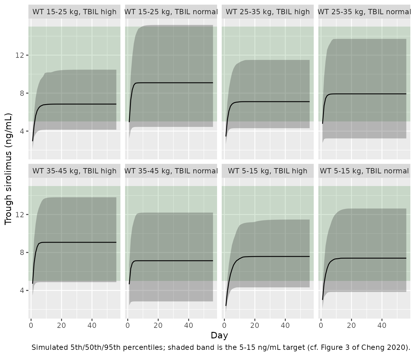
Table 4 - initial dose by body weight and total bilirubin
The paper does not report attainment probabilities for Table 4, so the table is checked two ways. First, a typical child at the midpoint of each weight band must have a steady-state trough inside 5-15 ng/mL on the recommended dose. The typical child has median total bilirubin (11.29 umol/L) in the normal band and 25 umol/L in the high band. Second, the table reports the simulated fraction of children whose steady-state trough falls in the target window.
# Closed-form steady-state trough of a one-compartment oral model, sampled
# 0.5 h before the next dose.
css_oral <- function(dose, cl, v, ka, tau, t) {
  k <- cl / v
  1000 * dose * ka / (v * (ka - k)) *
    (exp(-k * t) / (1 - exp(-k * tau)) - exp(-ka * t) / (1 - exp(-ka * tau)))
}
typ <- tab4 |>
  mutate(
    WT = (wt_lo + wt_hi) / 2,
    TBILI = ifelse(tbili_band == "normal", 11.29, 25),
    cl = exp(theta[["lcl"]]) * (TBILI / 11.29)^theta[["e_tbili_cl"]] * (WT / 28.5)^theta[["e_wt_cl"]],
    v = exp(theta[["lvc"]]),
    trough_typ = css_oral(dose_mg, cl, v, exp(theta[["lka"]]), tau, tau - 0.5)
  )

ss <- troughs |>
  filter(time == t_end - 0.5) |>
  group_by(cell) |>
  summarise(
    median_trough = median(Cc),
    pct_in_5_15 = 100 * mean(Cc >= 5 & Cc <= 15),
    pct_below_5 = 100 * mean(Cc < 5),
    pct_above_15 = 100 * mean(Cc > 15),
    .groups = "drop"
  )

typ |>
  select(cell, dose_mg, trough_typ) |>
  left_join(ss, by = "cell") |>
  dplyr::rename(
    "Table 4 cell" = cell, "Daily dose (mg)" = dose_mg,
    "Typical trough (ng/mL)" = trough_typ, "Median simulated trough" = median_trough,
    "% in 5-15" = pct_in_5_15, "% < 5" = pct_below_5, "% > 15" = pct_above_15
  ) |>
knitr::kable(digits = c(0, 2, 1, 1, 1, 1, 1))| Table 4 cell | Daily dose (mg) | Typical trough (ng/mL) | Median simulated trough | % in 5-15 | % < 5 | % > 15 |
|---|---|---|---|---|---|---|
| WT 5-15 kg, TBIL normal | 0.75 | 7.3 | 7.4 | 81.0 | 16.5 | 2.5 |
| WT 15-25 kg, TBIL normal | 1.50 | 9.3 | 9.1 | 88.0 | 6.5 | 5.5 |
| WT 25-35 kg, TBIL normal | 1.75 | 8.1 | 7.9 | 81.5 | 16.5 | 2.0 |
| WT 35-45 kg, TBIL normal | 2.00 | 7.4 | 7.1 | 80.0 | 19.0 | 1.0 |
| WT 5-15 kg, TBIL high | 0.50 | 6.7 | 7.6 | 88.5 | 10.5 | 1.0 |
| WT 15-25 kg, TBIL high | 0.75 | 6.5 | 6.8 | 85.0 | 14.5 | 0.5 |
| WT 25-35 kg, TBIL high | 1.00 | 6.6 | 7.1 | 87.0 | 12.5 | 0.5 |
| WT 35-45 kg, TBIL high | 1.50 | 8.1 | 9.1 | 90.0 | 7.0 | 3.0 |
# Deterministic typical-value check: every recommended dose puts the typical
# child of its cell inside the target window.
stopifnot(all(typ$trough_typ > 5 & typ$trough_typ < 15))
Every Table 4 dose puts the typical child of its cell inside the target window. The median simulated trough in each cell is close to the typical value, and most simulated children in each cell are in the window.
Closed-form check of the ODE solution
The ODE solution at steady state must match the closed-form trough for the same typical parameters. Both sides use the same parameters, so the only difference is numerical error, and the bound can be tight.
typ$id <- seq_len(nrow(typ))
ev_typ <- do.call(rbind, lapply(split(typ, typ$id), make_events))
ev_typ <- ev_typ[order(ev_typ$id, ev_typ$time, -ev_typ$evid), ]
sim_typ <- rxode2::rxSolve(rxode2::zeroRe(ui), ev_typ, returnType = "data.frame", omega = NA) |>
  filter(time == t_end - 0.5) |>
  arrange(id)
#> Warning: multi-subject simulation without without 'omega'
chk <- data.frame(ode = sim_typ$Cc, closed = typ$trough_typ)
chk$pct_diff <- 100 * (chk$ode - chk$closed) / chk$closed
knitr::kable(cbind(cell = typ$cell, round(chk, 4)))| cell | ode | closed | pct_diff |
|---|---|---|---|
| WT 5-15 kg, TBIL normal | 7.3153 | 7.3153 | 0e+00 |
| WT 15-25 kg, TBIL normal | 9.2704 | 9.2704 | 0e+00 |
| WT 25-35 kg, TBIL normal | 8.0953 | 8.0953 | 0e+00 |
| WT 35-45 kg, TBIL normal | 7.4321 | 7.4321 | 0e+00 |
| WT 5-15 kg, TBIL high | 6.6634 | 6.6635 | -1e-04 |
| WT 15-25 kg, TBIL high | 6.5050 | 6.5050 | 0e+00 |
| WT 25-35 kg, TBIL high | 6.6337 | 6.6337 | 0e+00 |
| WT 35-45 kg, TBIL high | 8.1463 | 8.1463 | 0e+00 |
PKNCA validation
PKNCA is run on the last dosing interval (1320-1344 h) of every simulated child, grouped by Table 4 cell. At steady state, AUC over one dosing interval equals Dose / CL for each individual, with the dose in mg and CL in L/h (times 1000 for ng.h/mL). This gives a per-subject identity. The only error is the trapezoidal error on the 0.5 h grid.
conc <- sim |>
  filter(time >= t_end - tau, !is.na(Cc)) |>
  select(id, time, Cc, cell)
dose_df <- events |>
  filter(evid == 1, time == t_end - tau) |>
  select(id, time, amt) |>
  left_join(subj |> select(id, cell), by = "id")

conc_obj <- PKNCA::PKNCAconc(conc, Cc ~ time | cell + id, concu = "ng/mL", timeu = "h")
dose_obj <- PKNCA::PKNCAdose(dose_df, amt ~ time | cell + id, doseu = "mg")
intervals <- data.frame(start = t_end - tau, end = t_end, auclast = TRUE, cmax = TRUE, cmin = TRUE, tmax = TRUE)
nca <- PKNCA::pk.nca(PKNCA::PKNCAdata(conc_obj, dose_obj, intervals = intervals))
nca_res <- as.data.frame(nca$result)

nca_res |>
  group_by(cell, PPTESTCD) |>
  summarise(median = median(PPORRES), .groups = "drop") |>
  tidyr::pivot_wider(names_from = PPTESTCD, values_from = median) |>
  dplyr::rename(
    "Table 4 cell" = cell, "AUCtau (ng.h/mL)" = auclast, "Cmax (ng/mL)" = cmax,
    "Cmin (ng/mL)" = cmin, "Tmax (h)" = tmax
  ) |>
knitr::kable(digits = 2)| Table 4 cell | AUCtau (ng.h/mL) | Cmax (ng/mL) | Cmin (ng/mL) | Tmax (h) |
|---|---|---|---|---|
| WT 15-25 kg, TBIL high | 218.44 | 11.04 | 6.77 | 3.5 |
| WT 15-25 kg, TBIL normal | 326.14 | 17.42 | 8.90 | 3.5 |
| WT 25-35 kg, TBIL high | 234.06 | 12.39 | 7.01 | 3.5 |
| WT 25-35 kg, TBIL normal | 296.17 | 17.14 | 7.77 | 3.5 |
| WT 35-45 kg, TBIL high | 308.94 | 17.03 | 8.90 | 3.5 |
| WT 35-45 kg, TBIL normal | 291.07 | 17.29 | 6.93 | 3.5 |
| WT 5-15 kg, TBIL high | 216.70 | 10.26 | 7.52 | 3.5 |
| WT 5-15 kg, TBIL normal | 223.00 | 11.36 | 7.31 | 3.5 |
# Per-subject identity AUCtau = 1000 * Dose / CL_i.
cl_i <- sim |>
  filter(time == t_end) |>
  select(id, cl)
auc_chk <- nca_res |>
  filter(PPTESTCD == "auclast") |>
  left_join(cl_i, by = "id") |>
  left_join(subj |> select(id, dose_mg), by = "id") |>
  mutate(expected = 1000 * dose_mg / cl, pct_diff = 100 * (PPORRES - expected) / expected)
stopifnot(nrow(auc_chk) == nrow(subj))
# Same drawn parameters on both sides; residual difference is trapezoidal error,
# plus a tiny carry-over for the slowest-clearing children.
stopifnot(abs(median(auc_chk$pct_diff)) < 0.5, quantile(abs(auc_chk$pct_diff), 0.9) < 1)
summary(auc_chk$pct_diff)
#>     Min.  1st Qu.   Median     Mean  3rd Qu.     Max.
#> -0.24756 -0.06745 -0.04774 -0.05401 -0.03423 -0.01451
Cheng 2020 reports no NCA parameters (all the data are troughs), so there is no published NCA to compare against. The PKNCA results are checked against the exact steady-state identity above.
Assumptions and deviations
- IIV scale. The abstract’s 3.53% and 7.27% are read as Phoenix omega^2 x 100 (log-scale variances 0.0353 and 0.0727). This is the same x100 convention the abstract uses for the residual term (Table 3 Sigma 0.22, written as “22.45%”). The literal-CV alternative is shown in the “Scale of the inter-individual variability” section. No result in the paper discriminates between them.
-
Residual error.
propSd = 0.2245uses the abstract’s more precise value. Table 3 rounds it to 0.22. - Ka. Ka is 0.7521 1/h (Methods) rather than the 0.75 printed in Table 3. The Methods value is the one that was held constant, and the Discussion quotes it as 0.752.
- Dosing interval. The Methods say sirolimus “was given orally daily”, so every simulation uses once-daily dosing. Table 4 doses are read as daily doses.
- Table 4 covariate distributions. Uniform draws within each band. The high-bilirubin band has no printed upper bound, and 40 umol/L is assumed. The typical-value check uses band-midpoint weights and 11.29 / 25 umol/L total bilirubin.
- Assay range. The Methods give the assay’s lower limit of quantification as 25 ng/mL, which is above the whole 5-15 ng/mL target range the troughs were titrated to. This is probably a typographical error (FPIA sirolimus assays usually quantify down to about 2.5 ng/mL). It has no effect on the model, which does not model censoring.
- Figure 3 (VPC) cannot be reproduced without the observed data. A simulated trough-percentile figure is shown instead.