Docetaxel, IV and oral with encequidar (Wang 2024)
Source:vignettes/articles/Wang_2024_docetaxel.Rmd
Wang_2024_docetaxel.RmdModel and source
- Citation: Wang D, Jackson C, Hung N, Hung T, Kwan R, Chan W-K, Qin A, Hughes-Medlicott NJ, Glue P, Duffull S. Oral docetaxel plus encequidar - a pharmacokinetic model and evaluation against IV docetaxel. J Pharmacokinet Pharmacodyn. 2024;51(4):335-. doi:10.1007/s10928-024-09913-y. Correction (author affiliations only): doi:10.1007/s10928-024-09924-9.
- Description: Three-compartment population PK model for total and unbound docetaxel in men with metastatic prostate cancer after a 1-h intravenous infusion of standard docetaxel and after a single dose of oral docetaxel taken 1 h after 15 mg of the P-glycoprotein inhibitor encequidar (oDox + E; Wang 2024). The disposition parameters are those of UNBOUND docetaxel: the central state holds the unbound-equivalent amount, so Cunbound = central / vc, and total plasma docetaxel is reconstructed as Cc = Cunbound / fu with a constant fraction unbound that differs between the intravenous formulation (fu 0.67%, polysorbate-80 micelle) and oDox + E (fu 1.02%), selected by ROUTE_IV. Oral absorption is first order with a lag time and a constant logit-normal bioavailability (F 25%). Residual error is combined additive plus proportional, estimated separately for each of the four route-by-analyte data sets. Nine patients; no covariates were tested.
- Article: https://doi.org/10.1007/s10928-024-09913-y
- Open-access full text and Supplementary file 1: https://www.ncbi.nlm.nih.gov/pmc/articles/PMC11254990/
Wang 2024 fitted one population PK model to total and unbound plasma docetaxel measured in the same nine men twice: once after their standard 1-h intravenous (IV) docetaxel infusion, and once after a single oral docetaxel dose taken 1 h after 15 mg of the intestinal P-glycoprotein inhibitor encequidar (“oDox + E”). The model was then used to ask whether any practical oDox + E regimen could match the unbound exposure of IV docetaxel (a GO / NO-GO decision).
The final model (Supplementary file 1, “Final Model (Combined)”
column, and the structure diagram in Supplement 2) is a
three-compartment model written for unbound docetaxel.
The central state therefore holds the unbound-equivalent amount,
Cunbound = central / vc, and total docetaxel is
reconstructed through a constant binding constant
B = 1 / fu. The fraction unbound differs between the two
formulations (0.67% for the polysorbate-80 IV product, 1.02% after oDox
+ E), so the packaged model takes the route as the covariate
ROUTE_IV. As the paper notes, total clearance is
CL * fu_iv = 8570 * 0.0067 = 57.3 L/h.
mod <- readModelDb("Wang_2024_docetaxel")
ui <- rxode2::rxode(mod)
#> ℹ parameter labels from comments will be replaced by 'label()'
th <- ui$theta
TV <- list(
  cl = exp(th[["lcl"]]), vc = exp(th[["lvc"]]),
  q = exp(th[["lq"]]), vp = exp(th[["lvp"]]),
  q2 = exp(th[["lq2"]]), vp2 = exp(th[["lvp2"]]),
  ka = exp(th[["lka"]]), tlag = exp(th[["ltlag"]]),
  fdepot = plogis(th[["logitfdepot"]]),
  fu_iv = exp(th[["lfu_iv"]]), fu_po = exp(th[["lfu_po"]])
)
str(TV)
#> List of 11
#>  $ cl    : num 8570
#>  $ vc    : num 3500
#>  $ q     : num 1250
#>  $ vp    : num 9450
#>  $ q2    : num 2810
#>  $ vp2   : num 61900
#>  $ ka    : num 0.223
#>  $ tlag  : num 0.242
#>  $ fdepot: num 0.25
#>  $ fu_iv : num 0.0067
#>  $ fu_po : num 0.0102
Population
Nine patients with metastatic prostate cancer who were receiving IV docetaxel completed the phase I open-label, two-period, two-treatment study (Wang 2024 Methods, “Study design”; trial reported by Jackson et al., reference 21 of the paper). The first period was the standard of care, about 75 mg/m^2 IV docetaxel over 1 h; the second, at least 3 weeks later, was a single oDox + E dose at 75, 150 or 300 mg/m^2. Total docetaxel was measured in every sample (24 after IV, 23 after oDox + E; LLOQ 2 ng/mL) and unbound docetaxel in 7 and 8 optimal-design-selected samples per patient (LLOQ 0.084 ng/mL; 25% below LLOQ, handled with the M6 method). The paper reports no age, weight or body surface area summary, and covariates were not tested because of the small sample.
The same information is available programmatically via
readModelDb("Wang_2024_docetaxel")()$population.
Source trace
All values come from the “Final Model (Combined)” column of Wang 2024 Supplementary file 1 (sub-model 6).
| Equation / parameter | Value | Source location |
|---|---|---|
lcl (unbound CL) |
log(8570 L/h) | Supplement 1, CL(/F) |
lvc |
log(3500 L) | Supplement 1, Vc |
lq |
log(1250 L/h) | Supplement 1, Qp1 |
lvp |
log(9450 L) | Supplement 1, Vp1 |
lq2 |
log(2810 L/h) | Supplement 1, Qp2 |
lvp2 |
log(61900 L) | Supplement 1, Vp2 |
lka |
log(0.223 1/h) | Supplement 1, ka |
ltlag |
log(0.242 h) | Supplement 1, ALAG |
logitfdepot |
logit(0.25) | Supplement 1, F = 25% |
lfu_iv |
log(0.0067) | Supplement 1, f unbound IV = 0.67% |
lfu_po |
log(0.0102) | Supplement 1, f unbound PO = 1.02% |
etalcl, etalka, etaltlag,
etalvc, etalvp
|
0.27^2, 0.47^2, 0.03^2, 0.63^2, 1.48^2 | Supplement 1, BSV CL 27%, ka 47%, ALAG 3%, Vc 63%, Vp1 148% |
etalogitfdepot |
0.71^2 | Supplement 1, BSV logitF = 0.71 (logit-scale SD) |
etalfu_iv, etalfu_po
|
0.28^2, 0.72^2 | Supplement 1, BSV BIV 28%, BPO 72% |
addSdIv, propSdIv
|
0.001 ng/mL, 0.143 | Supplement 1, Tot IV add ‘<0.001’, Tot IV prop |
addSdOral, propSdOral
|
0.199 ng/mL, 0.322 | Supplement 1, Tot PO add, Tot PO prop |
addSdIv_Cunbound, propSdIv_Cunbound
|
0.005 ng/mL, 0.538 | Supplement 1, UF IV add, UF IV prop |
addSdOral_Cunbound,
propSdOral_Cunbound
|
0.003 ng/mL, 0.337 | Supplement 1, UF PO add, UF PO prop |
| Three-compartment linear disposition of unbound drug, oral input with F, ka and lag | n/a | Results “Final model”; Supplement 2 |
Cc = Cunbound / fu, fu by route |
n/a | Supplement 1 abbreviations (fu = 1 / B); Supplement 2 |
Closed-form checks
The paper’s own derived quantity is total IV clearance, 57.3 L/h. A
typical patient’s unbound AUC after a dose is
F * Dose / CL, and total AUC is that divided by
fu.
cl_total_iv <- TV$cl * TV$fu_iv
cl_total_iv
#> [1] 57.419
stopifnot(abs(cl_total_iv - 57.3) / 57.3 < 0.01)

# Total steady-state volume implied by the tabulated parameters.
vss_total_iv <- (TV$vc + TV$vp + TV$vp2) * TV$fu_iv
vss_total_iv
#> [1] 501.495
The tabulated parameters give a total-docetaxel Vss of 501 L, against the 425 L quoted in the paper’s Discussion; the difference is discussed under Assumptions and deviations.
Virtual cohort
The trial doses were 75 mg/m^2 IV and 75, 150 or 300 mg/m^2 oDox + E. The paper’s own simulations convert 75 mg/m^2 to 130 mg using a body surface area of 1.7 m^2 (Table 2), and the same conversion is used here for every arm. Each virtual patient receives a single dose of one regimen.
set.seed(20240314)
n_per_arm <- 50L
bsa <- 1.7
arms <- tibble::tribble(
  ~treatment,               ~route_iv, ~dose_mgm2,
  "IV 75 mg/m^2",           1L,        75,
  "oDox+E 75 mg/m^2",       0L,        75,
  "oDox+E 150 mg/m^2",      0L,        150,
  "oDox+E 300 mg/m^2",      0L,        300
) |>
  mutate(amt = round(dose_mgm2 * bsa), arm = row_number())

obs_times <- sort(unique(c(seq(0, 2, by = 0.05), seq(2.25, 24, by = 0.25), seq(25, 168, by = 1))))

make_arm <- function(a) {
  ids <- (a$arm - 1L) * n_per_arm + seq_len(n_per_arm)
  dose <- tibble(
    id = ids, time = 0, amt = a$amt, evid = 1L,
    rate = if (a$route_iv == 1L) a$amt else 0,
    cmt = if (a$route_iv == 1L) "central" else "depot",
    dvid = NA_integer_
  )
  obs <- tidyr::expand_grid(id = ids, time = obs_times) |>
    mutate(amt = 0, evid = 0L, rate = 0, cmt = "central", dvid = 1L)
  bind_rows(dose, obs) |>
    mutate(treatment = a$treatment, ROUTE_IV = a$route_iv)
}

events <- bind_rows(lapply(split(arms, arms$arm), make_arm)) |>
  arrange(id, time, desc(evid))
stopifnot(!anyDuplicated(unique(events[, c("id", "time", "evid")])))Replicate published figures
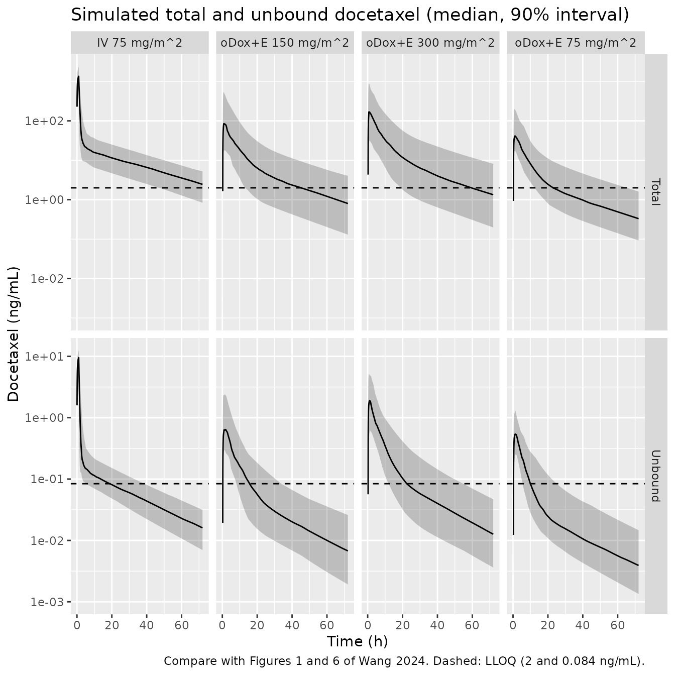
Figure 1 of Wang 2024 shows the observed total and unbound profiles of the nine patients; Figure 6 overlays the individual fits. The simulated 5th, 50th and 95th percentiles below should bracket those observations: IV total docetaxel peaks at roughly 1000-2000 ng/mL and unbound at about 5-15 ng/mL, while oDox + E total docetaxel peaks at roughly 50-200 ng/mL and unbound at about 0.3-2 ng/mL.
sim_pk |>
  filter(time <= 72) |>
  select(treatment, time, Cc, Cunbound) |>
  pivot_longer(c(Cc, Cunbound), names_to = "analyte", values_to = "conc") |>
  mutate(analyte = ifelse(analyte == "Cc", "Total", "Unbound")) |>
  group_by(treatment, analyte, time) |>
  summarise(
    Q05 = quantile(conc, 0.05), Q50 = quantile(conc, 0.50), Q95 = quantile(conc, 0.95),
    .groups = "drop"
  ) |>
  filter(Q50 > 0) |>
  ggplot(aes(time, Q50)) +
  geom_ribbon(aes(ymin = pmax(Q05, 1e-3), ymax = Q95), alpha = 0.25) +
  geom_line() +
  geom_hline(
    data = data.frame(analyte = c("Total", "Unbound"), lloq = c(2, 0.084)),
    aes(yintercept = lloq), linetype = "dashed"
  ) +
  facet_grid(analyte ~ treatment, scales = "free_y") +
  scale_y_log10() +
  labs(
    x = "Time (h)", y = "Docetaxel (ng/mL)",
    title = "Simulated total and unbound docetaxel (median, 90% interval)",
    caption = "Compare with Figures 1 and 6 of Wang 2024. Dashed: LLOQ (2 and 0.084 ng/mL)."
  )
peaks <- sim_pk |>
  group_by(treatment, id) |>
  summarise(cmax = max(Cc), cmax_u = max(Cunbound), .groups = "drop") |>
  group_by(treatment) |>
  summarise(median_cmax = median(cmax), median_cmax_unbound = median(cmax_u), .groups = "drop")
knitr::kable(peaks, digits = 2, caption = "Median simulated peak total and unbound docetaxel (ng/mL).")| treatment | median_cmax | median_cmax_unbound |
|---|---|---|
| IV 75 mg/m^2 | 1349.96 | 9.53 |
| oDox+E 150 mg/m^2 | 90.98 | 0.69 |
| oDox+E 300 mg/m^2 | 173.94 | 1.92 |
| oDox+E 75 mg/m^2 | 42.42 | 0.55 |
PKNCA validation
Wang 2024 reports no NCA table, so PKNCA is used here for two
purposes: to summarise the simulated exposure by arm for total and
unbound docetaxel, and to check the solver against each subject’s
closed-form unbound AUC0-inf, F_i * Dose / CL_i (F = 1 for
IV), using that subject’s own drawn parameters.
nca_input <- sim_pk |>
  select(id, time, treatment, Cc, Cunbound)
nca_input <- bind_rows(
  nca_input,
  nca_input |> distinct(id, treatment) |> mutate(time = 0, Cc = 0, Cunbound = 0)
) |>
  distinct(id, treatment, time, .keep_all = TRUE) |>
  arrange(id, treatment, time)

dose_df <- events |>
  filter(evid == 1) |>
  mutate(
    route = ifelse(ROUTE_IV == 1, "intravascular", "extravascular"),
    duration = ifelse(ROUTE_IV == 1, 1, 0)
  ) |>
  select(id, time, amt, treatment, route, duration)

intervals <- data.frame(
  start = 0, end = Inf,
  cmax = TRUE, tmax = TRUE, aucinf.obs = TRUE, half.life = TRUE
)

run_nca <- function(conc_col) {
  conc_df <- nca_input |>
    rename(conc = all_of(conc_col)) |>
    select(id, time, treatment, conc)
  conc_obj <- PKNCA::PKNCAconc(conc_df, conc ~ time | treatment + id,
                               concu = "ng/mL", timeu = "h")
  dose_obj <- PKNCA::PKNCAdose(dose_df, amt ~ time | treatment + id,
                               route = "route", duration = "duration", doseu = "mg")
  PKNCA::pk.nca(PKNCA::PKNCAdata(conc_obj, dose_obj, intervals = intervals))
}

nca_total <- run_nca("Cc")
nca_unbound <- run_nca("Cunbound")

summary(nca_total)
#>  Interval Start Interval End         treatment  N Cmax (ng/mL)
#>               0          Inf      IV 75 mg/m^2 50  1390 [37.3]
#>               0          Inf oDox+E 150 mg/m^2 50   90.2 [140]
#>               0          Inf oDox+E 300 mg/m^2 50    170 [150]
#>               0          Inf  oDox+E 75 mg/m^2 50  53.1 [97.8]
#>            Tmax (h) Half-life (h) AUCinf,obs (h*ng/mL)
#>   1.00 [1.00, 1.00]   29.0 [20.8]          2240 [42.6]
#>  1.12 [0.550, 2.50]   25.9 [15.9]            744 [121]
#>  1.00 [0.550, 3.00]   21.7 [8.34]           1260 [131]
#>  1.10 [0.500, 2.50]   21.9 [5.21]           376 [88.0]
#>
#> Caption: Cmax, AUCinf,obs: geometric mean and geometric coefficient of variation; Tmax: median and range; Half-life: arithmetic mean and standard deviation; N: number of subjects
summary(nca_unbound)
#>  Interval Start Interval End         treatment  N Cmax (ng/mL)
#>               0          Inf      IV 75 mg/m^2 50  9.63 [16.3]
#>               0          Inf oDox+E 150 mg/m^2 50 0.789 [84.1]
#>               0          Inf oDox+E 300 mg/m^2 50  1.93 [83.5]
#>               0          Inf  oDox+E 75 mg/m^2 50 0.558 [60.6]
#>            Tmax (h) Half-life (h) AUCinf,obs (h*ng/mL)
#>   1.00 [1.00, 1.00]   29.0 [20.8]          15.5 [23.6]
#>  1.12 [0.550, 2.50]   25.9 [15.9]          6.51 [69.7]
#>  1.00 [0.550, 3.00]   21.7 [8.34]          14.2 [70.9]
#>  1.10 [0.500, 2.50]   21.9 [5.21]          3.95 [57.8]
#>
#> Caption: Cmax, AUCinf,obs: geometric mean and geometric coefficient of variation; Tmax: median and range; Half-life: arithmetic mean and standard deviation; N: number of subjects
indiv <- sim |>
  group_by(id) |>
  summarise(cl = first(cl), fdepot = first(fdepot), .groups = "drop")
auc_check <- as.data.frame(nca_unbound) |>
  filter(PPTESTCD == "aucinf.obs") |>
  select(id, treatment, aucinf = PPORRES) |>
  left_join(dose_df |> select(id, amt), by = "id") |>
  left_join(indiv, by = "id") |>
  mutate(
    f = ifelse(grepl("^IV", treatment), 1, fdepot),
    auc_closed = f * amt / cl * 1000,
    pct_diff = 100 * (aucinf - auc_closed) / auc_closed
  )

auc_check |>
  group_by(treatment) |>
  summarise(
    median_pct_diff = median(pct_diff),
    q90_abs_pct_diff = quantile(abs(pct_diff), 0.9),
    .groups = "drop"
  ) |>
knitr::kable(digits = 2, caption = "PKNCA unbound AUC0-inf versus each subject's closed-form F * Dose / CL (percent difference).")| treatment | median_pct_diff | q90_abs_pct_diff |
|---|---|---|
| IV 75 mg/m^2 | -0.03 | 0.25 |
| oDox+E 150 mg/m^2 | -0.01 | 0.08 |
| oDox+E 300 mg/m^2 | 0.00 | 0.02 |
| oDox+E 75 mg/m^2 | -0.01 | 0.02 |
# Both sides use the same drawn parameters; the only differences are the
# trapezoidal AUC and the log-linear extrapolation past 168 h of a profile
# whose terminal half-life is about 21 h for a typical patient but can be
# much longer for a subject with a large Vp1.
stopifnot(
  abs(median(auc_check$pct_diff)) < 3,
  quantile(abs(auc_check$pct_diff), 0.9) < 10
)
GO / NO-GO probability of target attainment (Figures 7-9)
Wang 2024 compared each oDox + E regimen with 130 mg IV docetaxel
over 1 h in the same virtual patient. For each effective concentration
(EC) of unbound docetaxel from 0.1 to 1 ng/mL, the AUC of the unbound
profile above the EC (AUCOEC, Figure 2) was computed over 24 h on a
3-minute grid (Table 2). An oDox + E regimen succeeded for a patient
when its AUCOEC was at least 80% of that patient’s IV AUCOEC (a 20%
non-inferiority margin, Equation 1); the probability of target
attainment (PTA) is the share of successes (Equation 2). Two- and
three-dose regimens were evaluated by multiplying the single-dose AUCOEC
by the number of doses (complete washout between daily doses was
assumed). Unbound docetaxel does not depend on fu, so only
the disposition, absorption and bioavailability parameters matter here;
the paper simulated without residual error.
The paired design needs every regimen to share one patient’s random effects. The effects are therefore drawn in base R from the model’s omega matrix and passed to the typical-value model, so each virtual patient is solved once per regimen with identical parameters. The paper used 1000 virtual patients; 200 are used here.
set.seed(20240315)
n_pt <- 200L
omega <- ui$omega
eta <- matrix(rnorm(n_pt * nrow(omega)), n_pt) %*% chol(omega)
colnames(eta) <- rownames(omega)

regimens <- tibble::tribble(
  ~regimen,  ~route_iv, ~amt,
  "IV 130",  1L,        130,
  "PO 400",  0L,        400,
  "PO 450",  0L,        450,
  "PO 500",  0L,        500,
  "PO 550",  0L,        550,
  "PO 600",  0L,        600
) |>
  mutate(k = row_number())

grid24 <- seq(0, 24, by = 0.05)
pta_events <- bind_rows(lapply(seq_len(nrow(regimens)), function(r) {
  g <- regimens[r, ]
  ids <- (g$k - 1L) * n_pt + seq_len(n_pt)
  bind_rows(
    tibble(id = ids, time = 0, amt = g$amt, evid = 1L,
           rate = if (g$route_iv == 1L) g$amt else 0,
           cmt = if (g$route_iv == 1L) "central" else "depot", dvid = NA_integer_),
    tidyr::expand_grid(id = ids, time = grid24) |>
      mutate(amt = 0, evid = 0L, rate = 0, cmt = "central", dvid = 1L)
  ) |>
    mutate(regimen = g$regimen, patient = id - (g$k - 1L) * n_pt, ROUTE_IV = g$route_iv)
})) |>
  arrange(id, time, desc(evid))

pta_params <- pta_events |>
  distinct(id, patient) |>
  bind_cols(as.data.frame(eta[pta_events |> distinct(id, patient) |> pull(patient), , drop = FALSE])) |>
  select(-patient)

pta_sim <- rxode2::rxSolve(
  rxode2::zeroRe(mod), events = pta_events, params = pta_params,
  keep = c("regimen", "patient"), returnType = "data.frame"
) |>
  filter(!is.na(Cunbound))
#> ℹ parameter labels from comments will be replaced by 'label()'
#> Warning: No sigma parameters in the model
#> Warning: multi-subject simulation without without 'omega'
ec_levels <- seq(0.1, 1.0, by = 0.1)
trap_above <- function(time, conc, ec) {
  y <- pmax(conc - ec, 0)
  sum(diff(time) * (head(y, -1) + tail(y, -1)) / 2)
}
aucoec <- pta_sim |>
  group_by(regimen, patient) |>
  reframe(ec = ec_levels, aucoec = vapply(ec_levels, function(e) trap_above(time, Cunbound, e), numeric(1)))

target <- aucoec |>
  filter(regimen == "IV 130") |>
  transmute(patient, ec, target = 0.8 * aucoec)

pta <- aucoec |>
  filter(regimen != "IV 130") |>
  inner_join(target, by = c("patient", "ec")) |>
  tidyr::expand_grid(n_doses = 1:3) |>
  group_by(regimen, n_doses, ec) |>
  summarise(pta = 100 * mean(n_doses * aucoec >= target), .groups = "drop") |>
  mutate(dose_mg = as.numeric(sub("PO ", "", regimen)))
pta |>
  mutate(
    doses = factor(n_doses, labels = c("Single dose (Figure 7)", "Two doses (Figure 8)", "Three doses (Figure 9)")),
    dose_mg = factor(dose_mg)
  ) |>
  ggplot(aes(ec, pta, colour = dose_mg)) +
  geom_line() +
  geom_hline(yintercept = 80) +
  facet_wrap(~doses, ncol = 1) +
  scale_x_continuous(breaks = ec_levels) +
  labs(
    x = "Effective concentration (ng/mL)", y = "Probability of target attainment (%)",
    colour = "oDox + E dose (mg)",
    caption = "Replicates Figures 7, 8 and 9 of Wang 2024 (target: 130 mg IV docetaxel over 1 h)."
  )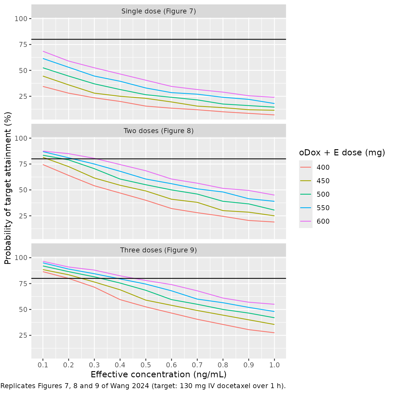
The maintainers digitised selected points from Figures 7-9 (read to about +/- 2 percentage points); the three-dose 600 mg value at 1 ng/mL (56%) is also printed in the Results, and the Discussion gives 74% for the single 600 mg dose.
published_pta <- tibble::tribble(
  ~n_doses, ~dose_mg, ~ec, ~pta_published,
  1L, 600, 0.1, 72.5,
  1L, 600, 0.3, 46,
  1L, 600, 0.5, 22.5,
  1L, 400, 0.1, 11,
  2L, 600, 0.1, 97.5,
  2L, 600, 0.3, 91,
  2L, 600, 0.5, 78.5,
  2L, 600, 0.7, 60,
  2L, 600, 1.0, 33.5,
  2L, 400, 0.1, 84.5,
  2L, 400, 0.3, 52.5,
  2L, 400, 0.5, 21.5,
  3L, 600, 0.3, 97,
  3L, 600, 0.5, 91,
  3L, 600, 0.7, 80,
  3L, 600, 1.0, 56,
  3L, 400, 0.1, 96.5,
  3L, 400, 0.3, 80.5,
  3L, 400, 0.5, 52,
  3L, 400, 1.0, 7
)

pta_cmp <- published_pta |>
  left_join(pta |> mutate(ec = round(ec, 1)), by = c("n_doses", "dose_mg", "ec")) |>
  mutate(difference = pta - pta_published)

pta_cmp |>
  select(n_doses, dose_mg, ec, pta_published, pta, difference) |>
  rename(
    "Doses" = n_doses, "oDox + E dose (mg)" = dose_mg, "EC (ng/mL)" = ec,
    "Published PTA (%)" = pta_published, "Simulated PTA (%)" = pta,
    "Difference (points)" = difference
  ) |>
knitr::kable(digits = 1, caption = "Simulated vs. published (digitised) PTA.")| Doses | oDox + E dose (mg) | EC (ng/mL) | Published PTA (%) | Simulated PTA (%) | Difference (points) |
|---|---|---|---|---|---|
| 1 | 600 | 0.1 | 72.5 | 68.5 | -4.0 |
| 1 | 600 | 0.3 | 46.0 | 52.5 | 6.5 |
| 1 | 600 | 0.5 | 22.5 | 40.5 | 18.0 |
| 1 | 400 | 0.1 | 11.0 | 34.5 | 23.5 |
| 2 | 600 | 0.1 | 97.5 | 87.5 | -10.0 |
| 2 | 600 | 0.3 | 91.0 | 80.5 | -10.5 |
| 2 | 600 | 0.5 | 78.5 | 68.5 | -10.0 |
| 2 | 600 | 0.7 | 60.0 | 56.5 | -3.5 |
| 2 | 600 | 1.0 | 33.5 | 45.0 | 11.5 |
| 2 | 400 | 0.1 | 84.5 | 74.5 | -10.0 |
| 2 | 400 | 0.3 | 52.5 | 54.0 | 1.5 |
| 2 | 400 | 0.5 | 21.5 | 40.0 | 18.5 |
| 3 | 600 | 0.3 | 97.0 | 88.0 | -9.0 |
| 3 | 600 | 0.5 | 91.0 | 78.0 | -13.0 |
| 3 | 600 | 0.7 | 80.0 | 68.0 | -12.0 |
| 3 | 600 | 1.0 | 56.0 | 55.0 | -1.0 |
| 3 | 400 | 0.1 | 96.5 | 86.5 | -10.0 |
| 3 | 400 | 0.3 | 80.5 | 71.5 | -9.0 |
| 3 | 400 | 0.5 | 52.0 | 52.5 | 0.5 |
| 3 | 400 | 1.0 | 7.0 | 27.5 | 20.5 |
# Gate only on the two values the paper prints in its text: 74% for a single
# 600 mg dose (Discussion; 72.5% at 0.1 ng/mL in Figure 7) and 56% for three
# 600 mg doses at 1 ng/mL (Results). The cohort is drawn with base R only, so
# it is the same on every machine; its Monte Carlo error at 200 patients is
# up to 3.5 points. A mis-read bioavailability or clearance moves either
# value by 15 points or more.
anchor_single <- pta_cmp |> filter(n_doses == 1L, dose_mg == 600, ec == 0.1)
anchor_triple <- pta_cmp |> filter(n_doses == 3L, dose_mg == 600, ec == 1.0)
stopifnot(
  abs(anchor_single$pta - 74) < 10,
  abs(anchor_triple$pta - 56) < 10
)
The two values printed in the text are reproduced, and so is the shape of the GO / NO-GO result: no single dose reaches 80% at any EC, while two or three daily 600 mg doses do at low EC. Away from those anchors the simulated curves are flatter across dose than the published ones: the 400 mg regimens attain the target more often at low EC and less often at high EC than in Figures 7-9, and the 600 mg multiple-dose regimens less often at intermediate EC (by up to about 20 points). The spread across dose at a fixed EC is driven almost entirely by the between-patient variability of the bioavailability, and simulating with the logit-scale SD of 0.71 tabulated in Supplement 1 gives a wider spread than the published curves imply, while removing that variability altogether gives a much narrower one. The paper’s simulation code is not published, so this is recorded as a known deviation rather than resolved by changing a tabulated value.
pta |>
  group_by(n_doses) |>
  summarise(max_pta = max(pta), .groups = "drop") |>
knitr::kable(digits = 1, caption = "Highest simulated PTA (%) over all doses and EC levels, by number of doses.")| n_doses | max_pta |
|---|---|
| 1 | 68.5 |
| 2 | 87.5 |
| 3 | 96.5 |
Assumptions and deviations
-
Unbound parameterisation. Supplement 1 states that
the parameters are “in the context of unbound docetaxel” and the Results
give total clearance as
CL * fu_iv; the central state therefore holds unbound-equivalent docetaxel and total concentration isCunbound / fu. -
Binding-constant variability. The paper places
exponential between-subject variability on the binding constants
B_IVandB_PO(B = 1 / fu). The model carries it onfuinstead;exp(eta)onBisexp(-eta)onfu, which is the same log-normal distribution. - Omega scale. The Supplement 1 footnote says the BSV values are CVs “calculated as the square root of the omega value”, so each variance is the square of the tabulated CV. The logit-F entry (0.71, no percent sign) is read as the SD on the logit scale. With it the single 600 mg dose comes close to the 74% PTA quoted in the Discussion (in closed form, at an effective concentration of zero, it gives exactly 74%).
- PTA curves. The simulated Figures 7-9 match the two PTA values printed in the text but are flatter across dose than the published curves (see the comparison table above); the paper’s simulation code is not available to explain the difference, and no tabulated value was changed.
- Vp2 variability. BSV on Vp2 was estimated at 0% (RSE NA) and is omitted.
- Residual error. The additive SD for total docetaxel after IV is tabulated as “<0.001” ng/mL; the bound 0.001 ng/mL is used (negligible next to the 14.3% proportional term at these concentrations). The combined error is encoded as nlmixr2’s standard additive-plus-proportional model; the paper does not state how the two terms were combined in NONMEM.
- Correlated residuals (L2). The final model let the residuals of the total and unbound measurements from the same blood sample be correlated (NONMEM L2 data item) but the correlation is not reported. The two outputs carry independent residual errors.
-
Total Vss. The Discussion quotes a total-docetaxel
Vss of 425 L; the tabulated volumes multiplied by
fu_ivgive about 502 L. The tabulated parameters are used unchanged, and they reproduce the paper’s 57.3 L/h total clearance exactly. - Body surface area. The paper reports no demographics; doses in mg/m^2 are converted with the 1.7 m^2 used in the paper’s own simulations.
- Oral docetaxel alone. The dashed “oral docetaxel alone (F = 8%)” curves of Figures 7-9 are not reproduced, because the paper does not say whether the bioavailability variability was kept when F was changed.
- Correction. A correction notice (doi:10.1007/s10928-024-09924-9) amends author affiliations only; no model value is affected.