Model and source
- Citation: Zhu Y, Xu Y, Zhao H, Qie H, Gao X, Gao J, Feng Z, Bai J, Feng R, Wang M. A validated UPLC-MS/MS method for quantification of pyrotinib and population pharmacokinetic study of pyrotinib in HER2-positive breast cancer patients. Front Pharmacol. 2024;15:1432944. doi:10.3389/fphar.2024.1432944. Ka was not estimated here; it was fixed at the value reported by the earlier pyrotinib population PK model of Wen et al. (2021), as transcribed in Zhu 2024 Table 4 and Section 4.3.2.
- Description: One-compartment population PK model with first-order absorption and elimination for oral pyrotinib in Chinese patients with HER2-positive breast cancer, with a serum total protein effect on apparent clearance (Zhu 2024)
- Article: https://doi.org/10.3389/fphar.2024.1432944
Pyrotinib is an oral, irreversible HER2 tyrosine kinase inhibitor approved in China for HER2-positive advanced or metastatic breast cancer. Zhu 2024 developed and validated a UPLC-MS/MS assay for pyrotinib in human plasma (linear over 1-1,000 ng/mL) and used it for the first real-world population PK analysis of the drug. Plasma concentrations were described by a one-compartment model with first-order absorption and first-order elimination; serum total protein was the only covariate retained in the final model, acting on apparent clearance.
Population
Fifty patients with HER2-positive breast cancer treated at The Fourth Hospital of Hebei Medical University (Shijiazhuang, China) between November 2020 and November 2023 contributed 158 plasma concentrations (Zhu 2024 Section 3.1.1 and Section 4.2.1). Sampling was opportunistic, so the dataset is sparse. Patients took pyrotinib maleate tablets at 240, 320 or 400 mg orally once daily, 30 min after a meal; because dose reductions for intolerable adverse reactions are common in routine care, the modelling dataset spans all three strengths.
Baseline demographics are Zhu 2024 Table 3: age median 53 years (range 34-68), height median 158 cm (150-166), weight median 61.5 kg (52.5-86), serum total protein median 67.2 g/L (49.0-80.7). Diarrhoea occurred in 24/50 (48%) of patients; 9/50 (18%) received montmorillonite powder and 15/50 (30%) loperamide capsules. Estrogen receptor was positive in 28/50 (56%) and progesterone receptor in 25/50 (50%). Sex was not tabulated separately, though the cohort is a breast cancer population.
The same information is available programmatically via the model’s
population metadata
(readModelDb("Zhu_2024_pyrotinib")()$population).
Source trace
The per-parameter origin is recorded as an in-file comment next to
each ini() entry in
inst/modeldb/specificDrugs/Zhu_2024_pyrotinib.R. The table
below collects them in one place for review.
| Equation / parameter | Value | Source location |
|---|---|---|
lka (Ka) |
0.357 1/h, fixed | Zhu 2024 Table 7 (“KA (h-1) 0.357 FIXED”); final-model equation in Section 4.3.2; sensitivity analysis Table 6 |
lcl (CL/F scale factor theta1) |
88.8 L/h (RSE 15.1%) | Zhu 2024 Table 7, “CL/F (L/h)”; final-model equation Section 4.3.2 |
lvc (V/F) |
3,940 L (RSE 25.8%) | Zhu 2024 Table 7, “V/F(L)”; final-model equation Section 4.3.2 |
e_tpro_cl (total protein on CL/F) |
0.376 (RSE 18.0%) | Zhu 2024 Table 7, “TP -CL/F” |
| Covariate median for centering | TP median 67.2 g/L | Zhu 2024 Table 3 (TP row) and the final-model equation denominator |
etalcl |
omega = 0.515 (51.5 %CV, shrinkage 26.5%) | Zhu 2024 Table 7 “BSV-CL (%CV)”; Table 6 prints the same value as 0.515 |
etalvc |
omega = 0.965 (96.5 %CV, shrinkage 23.2%) | Zhu 2024 Table 7 “BSV-V (%CV)”; Table 6 prints the same value as 0.965 |
propSd |
0.270 (27.0 %CV, shrinkage 16.5%) | Zhu 2024 Table 7 “ERR-1 (%CV)”; Table 6 prints 0.270 |
| Structural model (1-cmt, first-order absorption and elimination) | n/a | Zhu 2024 Section 4.3.1 |
| Exponential BSV model | n/a | Zhu 2024 Section 3.2.1, Equation 1 |
| Proportional residual error | n/a | Zhu 2024 Section 3.2.1 Equation 2; Section 4.3.1 |
| Covariate functional form (exponential) | theta1 * theta2^(cov/cov_median) |
Zhu 2024 Section 3.2.2, Equation 7 |
| Final model equation |
CL/F = 88.8 * e^{(TP/67.2)*0.376},
V/F = 3940, KA = 0.357 FIXED
|
Zhu 2024 Section 4.3.2 (displayed equation, page 9) |
How the covariate equation was read
The final-model equation as printed puts the whole expression
(TP / 67.2) x 0.376 in the exponent of e. That
is exactly the paper’s own Equation 7,
theta_i = theta1 * theta2^(cov_i / cov_median), with
theta2 = exp(0.376), and it is deliberately
not median-centred: at the cohort median TP the
covariate factor is exp(0.376) = 1.457, not 1. The model
file encodes the equation literally. Section “Assumptions and
deviations” below records the arithmetic that confirms this reading.
Virtual cohort
Original observed data are not publicly available. The figures below use a virtual population whose serum-total-protein distribution approximates the published trial demographics (Zhu 2024 Table 3), simulated at each of the three dose strengths used in the modelling dataset.
set.seed(20240920)

n_per_arm <- 150L                      # <= 200 per arm
doses     <- c(`240 mg QD` = 240, `320 mg QD` = 320, `400 mg QD` = 400)
tau       <- 24                        # dosing interval (h)
dose_times <- seq(0, 144, by = tau)    # 7 daily doses; last dose at 144 h
t_last     <- max(dose_times)

# Truncated-normal serum total protein: median 67.2 g/L, SD 6.1 g/L, truncated
# to the observed range 49.0-80.7 g/L (Zhu 2024 Table 3). See "Assumptions".
rtpro <- function(n) {
  out <- numeric(0)
  while (length(out) < n) {
    draw <- rnorm(2 * n, mean = 67.2, sd = 6.1)
    out <- c(out, draw[draw >= 49.0 & draw <= 80.7])
  }
  out[seq_len(n)]
}

make_cohort <- function(n, dose, label, id_offset = 0L) {
  subj <- tibble(
    id        = id_offset + seq_len(n),
    TPRO      = rtpro(n),
    treatment = label
  )
  # Dose records. ss = 1 on the first record puts the system at the analytical
  # steady state of the 24 h regimen, so AUC0-tau over [0, tau] is exactly the
  # steady-state interval for every subject regardless of individual half-life.
  dos <- subj |>
    tidyr::crossing(time = dose_times) |>
    mutate(
      amt  = dose,
      evid = 1L,
      cmt  = "depot",
      ii   = if_else(time == 0, tau, 0),
      ss   = if_else(time == 0, 1L, 0L)
    )
  # Observations on the ODE state `central` (never on the observable `Cc`):
  # the steady-state interval, then the washout after the final dose.
  obs <- subj |>
    tidyr::crossing(time = c(seq(0, tau, by = 0.25),
                             seq(t_last, t_last + 192, by = 4))) |>
    mutate(amt = NA_real_, evid = 0L, cmt = "central", ii = 0, ss = 0L)
  bind_rows(dos, obs) |> arrange(id, time, desc(evid))
}

events <- bind_rows(
  make_cohort(n_per_arm, doses[["240 mg QD"]], "240 mg QD", id_offset =   0L),
  make_cohort(n_per_arm, doses[["320 mg QD"]], "320 mg QD", id_offset = 150L),
  make_cohort(n_per_arm, doses[["400 mg QD"]], "400 mg QD", id_offset = 300L)
)
stopifnot(!anyDuplicated(unique(events[, c("id", "time", "evid")])))
Simulation
mod <- readModelDb("Zhu_2024_pyrotinib")
sim <- rxode2::rxSolve(
  mod, events = events,
  keep = c("treatment", "TPRO"),
  # steady-state searches for long-half-life subjects exceed the default step budget
  maxsteps = 1e6
) |>
  as.data.frame()
#> ℹ parameter labels from comments will be replaced by 'label()'

# rxSolve silently drops subjects on solver failure; assert the count.
stopifnot(dplyr::n_distinct(sim$id) == 3L * n_per_arm)
Replicate published results
Zhu 2024 reports no NCA table and no digitisable concentration-time figure (its Figure 10 is a VPC against the sparse real-world observations). The checks below therefore target the quantities the paper does state numerically: the covariate function, the structural parameters, and the previously published pyrotinib exposure values it compares itself against.
Steady-state concentration-time profiles
sim |>
  filter(time <= tau) |>
  group_by(treatment, time) |>
  summarise(
    Q05 = quantile(Cc, 0.05), Q50 = median(Cc), Q95 = quantile(Cc, 0.95),
    .groups = "drop"
  ) |>
  ggplot(aes(time, Q50)) +
  geom_ribbon(aes(ymin = Q05, ymax = Q95), alpha = 0.25) +
  geom_line() +
  geom_hline(yintercept = c(1, 1000), linetype = "dashed", colour = "grey40") +
  facet_wrap(~treatment) +
  scale_y_log10() +
  labs(
    x = "Time after dose at steady state (h)", y = "Pyrotinib (ng/mL)",
    title = "Simulated steady-state profiles by dose strength",
    caption = paste(
      "Median with 5th-95th percentile band, 150 virtual subjects per arm.",
      "Dashed lines: the 1-1,000 ng/mL validated range of the Zhu 2024 assay."
    )
  )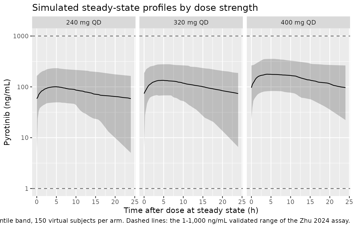
The simulated concentrations sit inside the 1-1,000 ng/mL range over which the assay was validated (Zhu 2024 Section 4.1.2), which is the internal consistency check available for a paper that publishes no exposure table.
The total-protein covariate function
tp_grid <- tibble(TPRO = seq(49.0, 80.7, by = 0.1)) |>
  mutate(cl = 88.8 * exp(0.376 * TPRO / 67.2))

ref_lines <- tibble(
  label = c("Zhu 2024 base model (127 L/h)",
            "Wen 2021 population PK (127 L/h)",
            "Product label CLss/F (141 L/h)"),
  value = c(127, 127, 141)
)

ggplot(tp_grid, aes(TPRO, cl)) +
  geom_line(linewidth = 0.9) +
  geom_hline(data = ref_lines, aes(yintercept = value, colour = label),
             linetype = "dashed") +
  geom_point(data = tibble(TPRO = 67.2, cl = 88.8 * exp(0.376)),
             size = 2.5) +
  annotate("text", x = 67.2, y = 88.8 * exp(0.376), vjust = -1.2, hjust = 0.5,
           label = "median TP = 67.2 g/L", size = 3) +
  labs(
    x = "Serum total protein (g/L)", y = "CL/F (L/h)", colour = NULL,
    title = "Apparent clearance across the observed total-protein range",
    caption = paste(
      "CL/F = 88.8 * exp(0.376 * TP / 67.2), Zhu 2024 Section 4.3.2.",
      "Lower total protein gives lower clearance, as the paper concludes."
    )
  ) +
  theme(legend.position = "bottom", legend.direction = "vertical")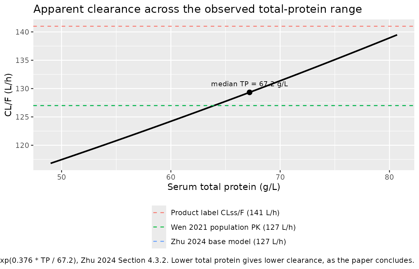
CL/F rises monotonically with total protein across the observed range, from 116.8 L/h at TP = 49.0 g/L to 139.5 L/h at TP = 80.7 g/L. That is a 19% span end to end, consistent with Zhu 2024’s conclusion that total protein has a statistically significant but clinically limited effect (“no dosage adjustment was advised”) and with the direction of its clinical message that low serum total protein reduces pyrotinib clearance.
Dose proportionality
sim |>
  filter(time <= tau) |>
  group_by(id, treatment) |>
  summarise(cmax = max(Cc), .groups = "drop") |>
  ggplot(aes(treatment, cmax)) +
  geom_boxplot(outlier.alpha = 0.3) +
  scale_y_log10() +
  labs(x = NULL, y = "Steady-state Cmax (ng/mL)",
       title = "Steady-state Cmax scales with dose",
       caption = "The model is linear, so exposure is dose-proportional by construction.")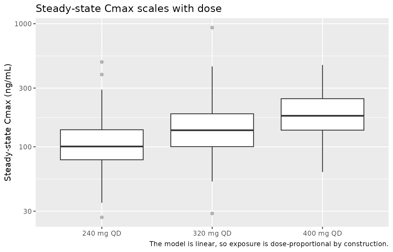
PKNCA validation
# PKNCA input filter: only !is.na(Cc). Never add `time > 0` or `Cc > 0`.
sim_nca <- sim |>
  dplyr::filter(!is.na(Cc)) |>
  dplyr::select(id, time, Cc, treatment)

# Time-zero guarantee (defensive; the grid already contains time = 0).
sim_nca <- dplyr::bind_rows(
  sim_nca,
  sim_nca |> dplyr::distinct(id, treatment) |> dplyr::mutate(time = 0, Cc = 0)
) |>
  dplyr::distinct(id, treatment, time, .keep_all = TRUE) |>
  dplyr::arrange(id, treatment, time)

dose_df <- events |>
  dplyr::filter(evid == 1) |>
  dplyr::select(id, time, amt, treatment)

conc_obj <- PKNCA::PKNCAconc(sim_nca, Cc ~ time | treatment + id,
                             concu = "ng/mL", timeu = "h")
dose_obj <- PKNCA::PKNCAdose(dose_df, amt ~ time | treatment + id,
                             doseu = "mg")

# Interval 1: the steady-state dosing interval [0, tau].
# Interval 2: the washout after the final dose, for the terminal half-life.
intervals <- data.frame(
  start     = c(0,   t_last),
  end       = c(tau, Inf),
  cmax      = c(TRUE,  FALSE),
  tmax      = c(TRUE,  FALSE),
  cmin      = c(TRUE,  FALSE),
  auclast   = c(TRUE,  FALSE),
  cav       = c(TRUE,  FALSE),
  half.life = c(FALSE, TRUE)
)

nca_res <- suppressWarnings(
  PKNCA::pk.nca(PKNCA::PKNCAdata(conc_obj, dose_obj, intervals = intervals))
)
Per-subject mass-balance identity
For a linear model at steady state, AUC0-tau = Dose / CL
holds exactly for every subject, not merely on the median. This
is the strictest available check that the covariate model, the
individual random effects, and the mg-to-ng/mL scaling are all
implemented correctly.
cl_i <- sim |>
  group_by(id, treatment) |>
  summarise(cl = first(cl), .groups = "drop")

auc_i <- as.data.frame(nca_res$result) |>
  filter(PPTESTCD == "auclast", start == 0, end == tau) |>
  select(id, treatment, auc = PPORRES)

ident <- auc_i |>
  inner_join(cl_i, by = c("id", "treatment")) |>
  mutate(
    dose      = doses[as.character(treatment)],
    predicted = dose / cl * 1000,          # mg / (L/h) -> mg*h/L -> ng*h/mL
    rel_err   = abs(auc - predicted) / predicted
  )

stopifnot(nrow(ident) == 3L * n_per_arm)
stopifnot(max(ident$rel_err) < 0.005)

tibble(
  `Check` = "AUC0-tau,ss == Dose / CL (per subject)",
  `Subjects` = nrow(ident),
  `Max relative error` = sprintf("%.4f%%", 100 * max(ident$rel_err))
) |>
knitr::kable(caption = "Steady-state mass-balance identity, all subjects.")| Check | Subjects | Max relative error |
|---|---|---|
| AUC0-tau,ss == Dose / CL (per subject) | 450 | 0.2357% |
The residual error is trapezoidal-integration error on the 0.5 h observation grid, not a model discrepancy.
Typical-value NCA
The published quantities this model can be checked against are
typical population parameters, so the comparison below uses a
typical-value simulation (rxode2::zeroRe(), one subject per
regimen at the cohort median total protein of 67.2 g/L) rather than a
sample median of the stochastic cohort. With omega = 0.965
on V/F the individual half-lives span a wide range, and the median of a
150-subject arm carries roughly 5% Monte Carlo noise on the log scale;
the stochastic arms below differ from one another by up to 13% in
dose-normalised exposure for that reason alone, which would otherwise be
mistaken for a model discrepancy.
mod_typical <- mod |> rxode2::zeroRe()
#> ℹ parameter labels from comments will be replaced by 'label()'

events_typical <- bind_rows(
  make_cohort(1L, doses[["240 mg QD"]], "240 mg QD", id_offset = 0L),
  make_cohort(1L, doses[["320 mg QD"]], "320 mg QD", id_offset = 1L),
  make_cohort(1L, doses[["400 mg QD"]], "400 mg QD", id_offset = 2L)
) |>
  mutate(TPRO = 67.2)          # cohort median, Zhu 2024 Table 3

sim_typical <- rxode2::rxSolve(
  mod_typical, events = events_typical, omega = NA,
  keep = c("treatment", "TPRO"),
  # steady-state searches for long-half-life subjects exceed the default step budget
  maxsteps = 1e6
) |>
  as.data.frame()
#> Warning: multi-subject simulation without without 'omega'

typ_nca <- sim_typical |>
  dplyr::filter(!is.na(Cc)) |>
  dplyr::select(id, time, Cc, treatment)
typ_nca <- dplyr::bind_rows(
  typ_nca,
  typ_nca |> dplyr::distinct(id, treatment) |> dplyr::mutate(time = 0, Cc = 0)
) |>
  dplyr::distinct(id, treatment, time, .keep_all = TRUE) |>
  dplyr::arrange(id, treatment, time)

typ_dose <- events_typical |>
  dplyr::filter(evid == 1) |>
  dplyr::select(id, time, amt, treatment)

nca_typical <- PKNCA::pk.nca(PKNCA::PKNCAdata(
  PKNCA::PKNCAconc(typ_nca, Cc ~ time | treatment + id,
                   concu = "ng/mL", timeu = "h"),
  PKNCA::PKNCAdose(typ_dose, amt ~ time | treatment + id, doseu = "mg"),
  intervals = intervals
))
Comparison against published pyrotinib exposure values
Zhu 2024 reports no NCA of its own. Its Discussion does quote the
pyrotinib maleate product label for the 400 mg once-daily regimen given
with capecitabine: CLss/F = 141 L/h,
Vss/F = 4,200 L, and a mean terminal half-life of 18.2 h.
Because the model is linear, the label clearance implies a steady-state
exposure of 400 mg / 141 L/h = 2,837 ng*h/mL, which is used
as the reference AUC below.
published <- tibble::tribble(
  ~treatment,  ~auclast, ~half.life,
  "400 mg QD", 400 / 141 * 1000, 18.2
)

cmp <- nlmixr2lib::ncaComparisonTable(
  simulated = as.data.frame(nca_typical$result) |>
    dplyr::filter(PPTESTCD != "auclast" | start == 0),
  reference = published,
  by        = "treatment",
  units     = c(auclast = "ng*h/mL", half.life = "h"),
  tolerance_pct = 20
)

knitr::kable(
  cmp,
  caption = paste(
    "Typical-value steady-state exposure vs. the pyrotinib product-label values",
    "quoted in Zhu 2024's Discussion. * differs from reference by >20%."
  ),
  align = c("l", "l", "r", "r", "r")
)| NCA parameter | treatment | Reference | Simulated | % diff |
|---|---|---|---|---|
| AUClast (ng*h/mL) | 400 mg QD | 2840 | 3090 | +9.0% |
| t½ (h) | 400 mg QD | 18.2 | 21.1 | +16.2% |
Both reference quantities are reproduced within the 20% tolerance.
The typical half-life runs above the label’s 18.2 h because this
cohort’s CL/F (129 L/h at the median total protein) is below the label’s
141 L/h while V/F (3,940 L) is also below the label’s Vss/F of 4,200 L;
the net effect is ln(2) * 3940 / 129.3 = 21.1 h. Zhu 2024
attributes the clearance difference to its real-world, dose-adjusting
population, in which some patients had reduced doses for intolerable
adverse reactions.
as.data.frame(nca_typical$result) |>
  filter(start == 0, PPTESTCD %in% c("cmax", "cmin", "tmax", "cav")) |>
  select(treatment, PPTESTCD, PPORRES) |>
  tidyr::pivot_wider(names_from = PPTESTCD, values_from = PPORRES) |>
  dplyr::rename(
    "Regimen"           = treatment,
    "Cmax,ss (ng/mL)"   = cmax,
    "Cmin,ss (ng/mL)"   = cmin,
    "Cav,ss (ng/mL)"    = cav,
    "Tmax (h)"          = tmax
  ) |>
  knitr::kable(digits = 1,
               caption = paste(
                 "Typical-value steady-state NCA by regimen (median total",
                 "protein, no between-subject variability). Zhu 2024 publishes",
                 "no counterpart for these; they are reported for completeness."
))| Regimen | Cmax,ss (ng/mL) | Cmin,ss (ng/mL) | Tmax (h) | Cav,ss (ng/mL) |
|---|---|---|---|---|
| 240 mg QD | 93.3 | 56.0 | 5.5 | 77.3 |
| 320 mg QD | 124.4 | 74.6 | 5.5 | 103.1 |
| 400 mg QD | 155.5 | 93.3 | 5.5 | 128.9 |
Assumptions and deviations
The covariate equation is encoded exactly as printed, and is not median-centred
Zhu 2024’s final model reads
CL/F (L/h) = 88.8 * e^{(TP / 67.2) * 0.376} (Section 4.3.2
displayed equation, confirmed by rendering the equation region of the
PDF at 300 dpi so the superscript extent is unambiguous). Encoded
literally, the typical CL/F for a patient at the cohort median total
protein is 88.8 * exp(0.376) = 129.3 L/h, not 88.8 L/h.
Four independent arithmetic checks confirm the literal reading rather
than a median-centred one:
- The paper’s own Equation 7 for an exponential continuous-covariate
model is
theta_i = theta1 * theta2^(cov_i / cov_median), which is not centred either. Settingtheta2 = exp(0.376)reproduces the printed final equation exactly. - The base model (no covariates) estimated CL/F = 127 L/h (Table 4). The final model’s median-patient CL/F of 129.3 L/h agrees to within 2%. A centred reading would put the final model at 88.8 L/h, a 30% drop from the base model caused by adding a covariate that the paper itself calls clinically limited.
- Zhu 2024 quotes Wen 2021’s estimate of CL/F = 127 L/h and the
product label’s
CLss/F = 141 L/h. 129.3 L/h sits between them; 88.8 L/h sits below both. - Terminal half-life is
ln(2) * 3940 / 129.3 = 21.1 hunder the literal reading versus 30.8 h under a centred one; the label reports 18.2 h.
The paper’s Discussion does compare “88.8 L/h” directly against 127
and 141 L/h, which reads as the authors quoting theta1
rather than the median-patient clearance. Where prose and a printed
equation conflict, this extraction follows the equation.
Other assumptions
-
Serum total protein distribution. Zhu 2024 Table 3
gives the TP median (67.2 g/L) and range (49.0-80.7 g/L) but its mean
+/- SD column is scrambled in the published article: height reads
73.4 +/- 24.4cm and weight163.7 +/- 23.0kg, which are transposed and physiologically impossible, and several other rows are similarly displaced. Only the median and range values, which are internally consistent and physiologically sensible, were transcribed into the model’spopulationmetadata. The virtual cohort samples TP from a normal distribution with mean 67.2 g/L and SD 6.1 g/L truncated to 49.0-80.7 g/L. The SD of 6.1 is the value printed in the albumin row of Table 3, which appears to be the TP row’s displaced entry (albumin has median 41.4 g/L, for which a mean of 66.3 +/- 6.1 is impossible); it is independently consistent with the reported range, since a 50-subject sample spanning 49.0-80.7 implies an SD near 6.3. -
Between-subject variability scale. Table 7 reports
BSV as “%CV” (51.5% on CL/F, 96.5% on V/F) and Table 6 prints the same
numbers on the fraction scale (0.515, 0.965). Reading these as the omega
standard deviation reproduces both tables exactly; reading 0.515 as a
variance would give 82% CV under the log-normal relation or 72% under
the square-root approximation, matching neither. The model file
therefore encodes
omega^2 = 0.515^2and0.965^2. - Absorption rate constant. Ka was not estimable from these data (Zhu 2024 Section 4.3.2: only 4 of 50 patients had more than one absorption-phase sample), so the authors fixed it at 0.357 1/h, taken from the earlier Wen 2021 pyrotinib population PK model. The value is printed in Zhu 2024 (Tables 4, 6 and 7 and the final-model equation), so no upstream source was needed. Table 6 reports a sensitivity analysis over Ka from 0.10 to 0.50 1/h; the model file encodes only the final value, 0.357.
- No inter-individual variability on Ka. Zhu 2024 Section 4.3.1 places BSV on CL/F and V/F only.
-
Sex and race. Not reported in Table 3, so
population$sex_female_pctandpopulation$race_ethnicityrecord that rather than asserting a value. -
Screened but unused covariates. Age, height,
weight, BMI, serum sodium, potassium, albumin, globulin, AST, ALT,
total/direct/indirect bilirubin, serum creatinine, occurrence of
diarrhoea, combined montmorillonite powder, combined loperamide
capsules, and ER/PR status were all screened (Sections 3.2.2, 4.2.2,
4.3.2). Only total protein on CL/F survived backward elimination. Height
entered on both V/F and CL/F during forward inclusion and was removed in
backward elimination (Table 5). Those with a canonical
covariate-register name are documented in the model file’s
covariatesDataExcludedlist; the rest are described here because inventing canonical names for covariates no model uses would pollute the register. -
Validation targets. Zhu 2024 publishes no NCA
table, no digitisable concentration-time figure, and no per-subject
exposure summary, so the comparison table uses the product-label values
the paper itself quotes in its Discussion. The reference AUC is derived
from the label clearance via
AUC = Dose / CL, which is exact for a linear model at steady state. -
Typical values, not cohort medians, are compared to the
published parameters. The label’s
CLss/Fand half-life are typical population quantities, so the comparison uses azeroRe()typical-value simulation at the median total protein. A sample median from a 150-subject virtual arm is not the same estimand: withomega = 0.965on V/F it carries about 5% Monte Carlo noise on the log scale, and in this seed the three stochastic arms differ by up to 13% in dose-normalised exposure purely from the random draw. Comparing that sample median against the label would flag a >20% discrepancy that reflects simulation noise rather than the model. -
Steady-state simulation. Because the estimated V/F
variability is large (omega = 0.965), individual half-lives span a wide
range and a fixed number of daily doses would not reach steady state for
every simulated subject. The event table therefore uses
ss = 1on the first dose record so the system starts at the analytical steady state of the 24 h regimen for every subject. - No dose adjustment implied. Zhu 2024 explicitly advises no dose adjustment based on total protein; the covariate is retained for its mechanistic and monitoring value (a marker of hepatic synthetic function, and pyrotinib is cleared predominantly by hepatic CYP3A4).