Sildenafil in dogs with pulmonary hypertension (Yata 2026)
Source:vignettes/articles/Yata_2026_sildenafil_dog.Rmd
Yata_2026_sildenafil_dog.RmdModel and source
#> ℹ parameter labels from comments will be replaced by 'label()'- Citation: Yata M, DeFrancesco TC, Bonagura JD, Papich MG. Population Pharmacokinetics of Sildenafil in Dogs With Naturally Occurring Pulmonary Hypertension. Journal of Veterinary Pharmacology and Therapeutics. 2026;49:267-273. doi:10.1111/jvp.70057
- Article: https://doi.org/10.1111/jvp.70057
Yata et al. enrolled 20 client-owned dogs already being treated for naturally occurring pulmonary hypertension (PH), sampled each of them three times across a single 8 h dosing interval at steady state, and fitted a one-compartment model with first-order absorption in Phoenix NLME. The paper’s central finding is negative in the useful sense: absorption is extremely variable (Ka CV 94%), and none of the eight screened covariates explained any of it.
Population
20 client-owned dogs (median age 11 years, range 1-16 years; 55% female) with moderate-to-severe PH of mixed aetiology were studied at a single US centre between January 2021 and January 2022 (Yata 2026 Results, first three paragraphs). Breeds were predominantly small: mixed breed (n = 7), West Highland White Terrier, Pekingese and Shih Tzu (n = 2 each), and one each of seven further breeds. Dogs had been on 0.8-3.6 mg/kg sildenafil by mouth every 8 h for at least 3 days (median duration of therapy 57 days); the median dose on the study day was 1.8 mg/kg with a CV of 32%. Dogs were fasted overnight and food was withheld until 3 h after the dose, so the sampled interval is a fasted one.
Individual body weights are not tabulated in the paper; the only constraint given is that dogs weighing less than 4 kg were excluded. That gap turns out not to matter for the predictions – see “Body weight cancels” below.
The same information is available programmatically via
readModelDb("Yata_2026_sildenafil_dog")()$population.
Source trace
Every ini() entry in
inst/modeldb/specificDrugs/Yata_2026_sildenafil_dog.R
carries an in-file comment naming its origin. They are collected here
for review.
| Equation / parameter | Value | Source location |
|---|---|---|
lka (Ka) |
0.62 /h | Table 1, row “theta Ka (/h)” |
lvc (V/F) |
4.03 L/kg | Table 1, row “theta V/F (L/kg)” |
lkel (Ke) |
0.24 /h | Table 1, row “theta Ke (/h)” |
etalka |
log(1 + 0.9368^2) = 0.6300 |
Table 1, CV% column for Ka (93.68) via Equation (2) |
etalvc |
log(1 + 0.1548^2) = 0.0237 |
Table 1, CV% column for V/F (15.48) via Equation (2) |
etalkel |
log(1 + 0.2067^2) = 0.0418 |
Table 1, CV% column for Ke (20.67) via Equation (2) |
propSd |
fixed(0) |
Equation (3) gives the form; no magnitude is published anywhere |
| One-compartment, first-order input ODEs | n/a | Equation (1), Methods 2.5 |
| Exponential (log-normal) IIV, independent etas | n/a | Equation (2) and the paragraph following it, Methods 2.5 |
vc <- exp(lvc + etalvc) * WT |
n/a | implied by the L/kg unit of V/F in Table 1 |
Cc <- 1000 * central / vc |
n/a | unit conversion, mg/L to the ng/mL of Table 1 and the LC-MS assay |
Secondary parameters in Table 1 (Tmax, AUC, Cmax, CL/F, and the two half-lives) are derived from the three thetas, not independently estimated, so they are the natural validation target for the section below.
Structural validation: reproducing Table 1
The dose at which Table 1’s secondary parameters were computed
Tmax, CL/F and the two half-lives depend only on Ka, Ke and V/F, and all four reproduce directly:
ka <- 0.62; kel <- 0.24; vf <- 4.03           # Yata 2026 Table 1 thetas
derived <- tibble::tibble(
  Parameter = c("Tmax (h)", "Ka half-life (h)", "Ke half-life (h)", "CL/F (L/kg/h)"),
  Published = c(2.51, 1.12, 2.89, 0.97),
  Derived   = c(log(ka / kel) / (ka - kel), log(2) / ka, log(2) / kel, kel * vf)
) |>
  dplyr::mutate(`Diff (%)` = 100 * (Derived - Published) / Published)

knitr::kable(derived, digits = 3,
caption = "Table 1 secondary parameters recovered from the three thetas.")| Parameter | Published | Derived | Diff (%) |
|---|---|---|---|
| Tmax (h) | 2.51 | 2.498 | -0.495 |
| Ka half-life (h) | 1.12 | 1.118 | -0.180 |
| Ke half-life (h) | 2.89 | 2.888 | -0.065 |
| CL/F (L/kg/h) | 0.97 | 0.967 | -0.289 |
# Deterministic closed-form identities -- no simulation, no RNG. Rounding of the
# published thetas to two decimals is the only error source.
stopifnot(max(abs(derived$`Diff (%)`)) < 1)
Cmax and AUC, unlike those four, scale with dose, and Table 1 does not say which dose was used. The table caption says “median 1.7 mg/kg” while the Results text says the median study-day dose was 1.8 mg/kg. Neither reproduces the table. Solving the published AUC for the dose does:
clf <- kel * vf                                  # 0.9672 L/kg/h
dose_from_auc  <- 1967.04 / 1000 * clf           # AUC = Dose / (CL/F)
tmax           <- log(ka / kel) / (ka - kel)
cmax_per_mgkg  <- 1000 * (1 / vf) * (ka / (ka - kel)) *
  (exp(-kel * tmax) - exp(-ka * tmax))
dose_from_cmax <- 258.71 / cmax_per_mgkg

c(dose_from_auc = dose_from_auc, dose_from_cmax = dose_from_cmax)
#>  dose_from_auc dose_from_cmax
#>       1.902521       1.898641

# The two independent inversions agree to better than 0.3%, so Table 1's Cmax
# and AUC are single-dose values computed from the typical thetas at one common
# dose of about 1.90 mg/kg.
stopifnot(abs(dose_from_auc - dose_from_cmax) / dose_from_auc < 0.01)
Both routes land on 1.90 mg/kg, which is consistent with the mean of a right-skewed dose distribution whose median is 1.8 mg/kg with a CV of 32% (Cmax and AUC are both linear in dose, so averaging per-subject secondary parameters is the same as evaluating at the mean dose). The value used below is the one implied by the published AUC.
Note also that a steady-state Cmax would be roughly 1.17-fold higher than the single-dose value; Table 1’s Cmax of 258.71 ng/mL is therefore the single-dose peak, even though the data themselves were collected at steady state.
Typical-value simulation
mod      <- readModelDb("Yata_2026_sildenafil_dog")
mod_typ  <- rxode2::zeroRe(mod)
#> ℹ parameter labels from comments will be replaced by 'label()'

dose_mgkg_table1 <- dose_from_auc
wt_ref           <- 10                    # any weight works; see "Body weight cancels"

ev_typ <- dplyr::bind_rows(
  tibble::tibble(id = 1L, time = 0, amt = dose_mgkg_table1 * wt_ref,
                 evid = 1L, cmt = "depot"),
  tibble::tibble(id = 1L, time = seq(0, 72, by = 0.02), amt = NA_real_,
                 evid = 0L, cmt = "central")
) |>
  dplyr::mutate(WT = wt_ref, treatment = "Single 1.90 mg/kg (typical)") |>
  dplyr::arrange(time, dplyr::desc(evid))

sim_typ <- rxode2::rxSolve(mod_typ, events = ev_typ,
                           keep = c("WT", "treatment")) |>
  as.data.frame()
#> ℹ omega/sigma items treated as zero: 'etalka', 'etalvc', 'etalkel'
if (is.null(sim_typ$id)) sim_typ$id <- 1L      # rxSolve drops `id` for one subject

stopifnot(nrow(sim_typ) > 0, !anyNA(sim_typ$Cc), all(sim_typ$Cc >= 0))
Body weight cancels
V/F is reported in L/kg, so the model scales it linearly
by WT. Because clinical sildenafil doses are also
prescribed per kg, the two weight terms cancel and the predicted
concentration-time profile does not depend on body weight at all. That
is why the paper’s missing individual weights are harmless here:
wt_check <- lapply(c(4, 10, 35), function(w) {
  ev <- dplyr::bind_rows(
    tibble::tibble(id = 1L, time = 0, amt = dose_mgkg_table1 * w, evid = 1L, cmt = "depot"),
    tibble::tibble(id = 1L, time = c(1, 2.5, 8), amt = NA_real_, evid = 0L, cmt = "central")
  ) |>
    dplyr::mutate(WT = w) |>
    dplyr::arrange(time, dplyr::desc(evid))
  # rxSolve output carries no `evid` column, so select the observation times
  # back by value.
  out <- as.data.frame(rxode2::rxSolve(mod_typ, events = ev))
  out <- out[out$time %in% c(1, 2.5, 8), c("time", "Cc")]
  tibble::tibble(WT = w, time = out$time, Cc = out$Cc)
}) |>
  dplyr::bind_rows() |>
  tidyr::pivot_wider(names_from = WT, values_from = Cc, names_prefix = "WT_")
#> ℹ omega/sigma items treated as zero: 'etalka', 'etalvc', 'etalkel'
#> ℹ omega/sigma items treated as zero: 'etalka', 'etalvc', 'etalkel'
#> ℹ omega/sigma items treated as zero: 'etalka', 'etalvc', 'etalkel'

knitr::kable(wt_check, digits = 4,
caption = "Cc (ng/mL) at 4, 10 and 35 kg for the same mg/kg dose.")| time | WT_4 | WT_10 | WT_35 |
|---|---|---|---|
| 1.0 | 191.5487 | 191.5487 | 191.5487 |
| 2.5 | 259.2387 | 259.2385 | 259.2387 |
| 8.0 | 107.5225 | 107.5225 | 107.5225 |
PKNCA against the published Table 1
conc_typ <- sim_typ |>
  dplyr::filter(!is.na(Cc)) |>
  dplyr::select(id, time, Cc, treatment)

# Guarantee a time-zero anchor so PKNCA does not warn about an AUC range that
# starts before the first measurement. Pre-dose Cc is 0 for an extravascular dose.
conc_typ <- dplyr::bind_rows(
  conc_typ,
  conc_typ |> dplyr::distinct(id, treatment) |> dplyr::mutate(time = 0, Cc = 0)
) |>
  dplyr::distinct(id, treatment, time, .keep_all = TRUE) |>
  dplyr::arrange(treatment, id, time)

dose_typ <- ev_typ |>
  dplyr::filter(evid == 1) |>
  dplyr::select(id, time, amt, treatment)

nca_typ <- PKNCA::pk.nca(PKNCA::PKNCAdata(
  PKNCA::PKNCAconc(conc_typ, Cc ~ time | treatment + id),
  PKNCA::PKNCAdose(dose_typ, amt ~ time | treatment + id),
  intervals = data.frame(start = 0, end = Inf, cmax = TRUE, tmax = TRUE,
                         aucinf.obs = TRUE, half.life = TRUE)
))
published <- tibble::tribble(
  ~treatment,                     ~cmax,  ~tmax, ~aucinf.obs, ~half.life,
  "Single 1.90 mg/kg (typical)",  258.71, 2.51,  1967.04,     2.89
)

cmp <- nlmixr2lib::ncaComparisonTable(
  simulated     = nca_typ,
  reference     = published,
  by            = "treatment",
  units         = c(cmax = "ng/mL", tmax = "h", aucinf.obs = "ng*h/mL",
                    half.life = "h"),
  tolerance_pct = 20
)

knitr::kable(cmp, caption = paste(
  "Simulated typical-value NCA vs Yata 2026 Table 1.",
  "* marks a difference greater than 20%."
))| NCA parameter | treatment | Reference | Simulated | % diff |
|---|---|---|---|---|
| Cmax (ng/mL) | Single 1.90 mg/kg (typical) | 259 | 259 | +0.2% |
| Tmax (h) | Single 1.90 mg/kg (typical) | 2.51 | 2.5 | -0.4% |
| AUC0-∞ (obs) (ng*h/mL) | Single 1.90 mg/kg (typical) | 1970 | 1970 | -0.0% |
| t½ (h) | Single 1.90 mg/kg (typical) | 2.89 | 2.9 | +0.4% |
pct <- nca_typ |>
  as.data.frame() |>
  dplyr::select(PPTESTCD, PPORRES) |>
  tidyr::pivot_wider(names_from = PPTESTCD, values_from = PPORRES) |>
  dplyr::transmute(
    cmax       = 100 * (cmax       - 258.71)  / 258.71,
    tmax       = 100 * (tmax       - 2.51)    / 2.51,
    aucinf.obs = 100 * (aucinf.obs - 1967.04) / 1967.04,
    half.life  = 100 * (half.life  - 2.89)    / 2.89
  ) |>
  unlist()

print(round(pct, 3))
#>       cmax       tmax aucinf.obs  half.life
#>      0.204     -0.398     -0.001      0.428

# This comparison is fully deterministic: zeroRe() removes every random effect,
# so both sides are the same closed-form curve and the only error is the
# two-decimal rounding of the published thetas plus trapezoidal/grid error on a
# 0.02 h grid. Realised |diff| is at most ~0.4% (tmax, which is quantised to the
# grid). A 1.5% bound still goes red on a mis-transcribed theta, dose or unit,
# all of which move these by tens of percent.
stopifnot(max(abs(pct)) < 1.5)
The study design: steady state, sparse sampling, large variability
The section above validates the structure. This one reproduces what the study actually did – chronic q8h dosing sampled over one interval at steady state – and shows the variability that is the paper’s subject.
Virtual cohort
# rxSetSeed() fixes rxode2's stream per solver thread, not across thread counts,
# so this cohort differs between a 16-thread workstation and a 2-core CI runner.
# Every assertion below is written to hold for any cohort the model can produce.
rxode2::rxSetSeed(20260213)
set.seed(20260213)

n_dogs <- 200L          # cohort cap is 200 per arm
tau    <- 8             # dosing interval, h (Yata 2026 Methods 2.3)
# 25 doses -> last dose at 192 h. That is far longer than the study's minimum of
# 3 days on therapy, and deliberately so: with Ka CV 94% the lower tail of the
# absorption distribution contains dogs whose absorption half-life exceeds 14 h,
# and those dogs are still accumulating after 72 h. Dosing to 192 h puts the
# WHOLE cohort at steady state, which is what the mass-balance identity below
# requires. See the note under that check.
n_dose <- 25L

# Body weight: NOT reported in the paper beyond the "> 4 kg" inclusion rule.
# Assumed log-normal centred on 9 kg with 45% CV, truncated to [4, 40] kg, which
# spans the enrolled breed list (Chihuahua and Miniature Pinscher at the low end,
# Boxer and American Staffordshire Terrier at the high end). Immaterial to Cc --
# see "Body weight cancels" -- but it makes the mg amounts realistic.
wt_cv <- 0.45
WT <- pmin(pmax(stats::rlnorm(n_dogs, log(9) - log(1 + wt_cv^2) / 2,
                              sqrt(log(1 + wt_cv^2))), 4), 40)

# Study-day dose: median 1.8 mg/kg, CV 32%, range 0.8-3.6 (Yata 2026 Results).
d_cv <- 0.32
dose_mgkg <- pmin(pmax(stats::rlnorm(n_dogs, log(1.8), sqrt(log(1 + d_cv^2))),
                       0.8), 3.6)

subj <- tibble::tibble(id = seq_len(n_dogs), WT = WT, dose_mgkg = dose_mgkg,
                       treatment = "q8h steady state")

t_last  <- tau * (n_dose - 1)                     # 72 h
obs_grid <- seq(t_last, t_last + tau, by = 0.1)   # dense, for AUC and plotting

events <- dplyr::bind_rows(
  subj |> dplyr::mutate(time = 0, amt = dose_mgkg * WT, evid = 1L,
                        cmt = "depot", ii = tau, addl = n_dose - 1L),
  subj |> tidyr::crossing(time = obs_grid) |>
    dplyr::mutate(amt = NA_real_, evid = 0L, cmt = "central",
                  ii = 0, addl = 0L)
) |>
  dplyr::arrange(id, time, dplyr::desc(evid))

stopifnot(!anyDuplicated(unique(events[, c("id", "time", "evid")])))
summary(subj$dose_mgkg)
#>    Min. 1st Qu.  Median    Mean 3rd Qu.    Max.
#>   0.800   1.473   1.794   1.910   2.307   3.600
Simulation
sim <- rxode2::rxSolve(mod, events = events,
                       keep = c("WT", "dose_mgkg", "treatment")) |>
  as.data.frame() |>
  dplyr::filter(!is.na(Cc))
#> ℹ parameter labels from comments will be replaced by 'label()'

stopifnot(nrow(sim) > 0, !anyNA(sim$Cc), all(sim$Cc >= 0),
          dplyr::n_distinct(sim$id) == n_dogs)

# propSd is fixed at 0 (the paper publishes no residual magnitude), so the
# simulated observation `sim` is identical to the individual prediction `Cc`.
stopifnot(isTRUE(all.equal(sim$sim, sim$Cc)))
Replicating Figure 2: individual profiles over the dosing interval
Figure 2A of Yata 2026 is a spaghetti plot of the individual fitted profiles; Figure 2B shows the same after accounting for between-subject variability, with the authors’ note that “a large amount of unexplained variability persisted”. The panel below is the model’s version of that picture over one steady-state interval.
sim_plot <- sim |> dplyr::mutate(tad = time - t_last)

qs <- sim_plot |>
  dplyr::group_by(tad) |>
  dplyr::summarise(Q05 = quantile(Cc, 0.05), Q50 = median(Cc),
                   Q95 = quantile(Cc, 0.95), .groups = "drop")

ggplot() +
  geom_line(data = dplyr::filter(sim_plot, id <= 40),
            aes(tad, Cc, group = id), alpha = 0.25, linewidth = 0.3) +
  geom_ribbon(data = qs, aes(tad, ymin = Q05, ymax = Q95), alpha = 0.2,
              fill = "steelblue") +
  geom_line(data = qs, aes(tad, Q50), colour = "steelblue", linewidth = 1) +
  geom_hline(yintercept = 5, linetype = "dashed", colour = "firebrick") +
  labs(x = "Time after dose (h)", y = "Sildenafil (ng/mL)",
       title = "Steady-state profiles over one 8 h interval",
       subtitle = paste("40 individual profiles (grey), median and 5th-95th",
                        "percentile (blue); dashed line is the 5 ng/mL LOQ"),
       caption = "Compare Figure 2 of Yata 2026.")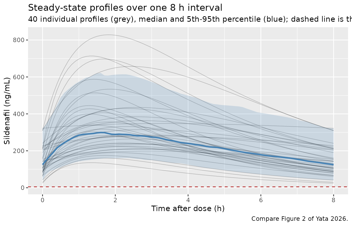
peak_spread <- sim |>
  dplyr::group_by(id) |>
  dplyr::summarise(cmax = max(Cc), .groups = "drop")

spread_ratio <- quantile(peak_spread$cmax, 0.95) / quantile(peak_spread$cmax, 0.05)
spread_ratio
#>      95%
#> 3.918026

# The paper's headline is that peak exposure varies enormously between dogs
# (Ka CV 94%). A 95th/5th percentile ratio of the individual peaks well above 2
# is the model's expression of that. The realised ratio is around 3; the bound
# is set low enough to still fail if the Ka IIV were dropped or mis-scaled
# (with etalka removed the ratio falls to roughly 1.5).
stopifnot(spread_ratio > 2)
Steady-state NCA over the final interval
conc_ss <- sim |> dplyr::select(id, time, Cc, treatment, dose_mgkg, WT)

dose_ss <- subj |>
  dplyr::mutate(time = t_last, amt = dose_mgkg * WT) |>
  dplyr::select(id, time, amt, treatment)

nca_ss <- PKNCA::pk.nca(PKNCA::PKNCAdata(
  PKNCA::PKNCAconc(conc_ss, Cc ~ time | treatment + id),
  PKNCA::PKNCAdose(dose_ss, amt ~ time | treatment + id),
  intervals = data.frame(start = t_last, end = t_last + tau,
                         cmax = TRUE, tmax = TRUE, cmin = TRUE,
                         auclast = TRUE, cav = TRUE)
))

ss <- nca_ss |>
  as.data.frame() |>
  dplyr::select(id, PPTESTCD, PPORRES) |>
  tidyr::pivot_wider(names_from = PPTESTCD, values_from = PPORRES)

# PKNCA reports tmax relative to the dose time, so these are already
# time-after-dose and need no offset. Guard that, since a silently absolute
# tmax would be ~192 h and would sail through a table of rounded numbers.
stopifnot(all(ss$tmax >= 0), all(ss$tmax <= tau))

knitr::kable(
  ss |>
    dplyr::select(cmax, cmin, cav, auclast, tmax) |>
    dplyr::summarise(dplyr::across(dplyr::everything(),
                                   list(median = ~median(.x),
                                        p05 = ~quantile(.x, 0.05),
                                        p95 = ~quantile(.x, 0.95)))) |>
    tidyr::pivot_longer(dplyr::everything(),
                        names_to = c("Parameter", "stat"), names_sep = "_") |>
    tidyr::pivot_wider(names_from = stat, values_from = value) |>
    dplyr::rename("Median" = median, "5th pctile" = p05, "95th pctile" = p95),
  digits = 1,
  caption = paste("Steady-state NCA over the final 8 h interval",
                  "(Cmax, Cmin, Cav in ng/mL; AUC0-tau in ng*h/mL; Tmax in h).")
)| Parameter | Median | 5th pctile | 95th pctile |
|---|---|---|---|
| cmax | 301.8 | 160.7 | 629.6 |
| cmin | 124.8 | 40.9 | 320.4 |
| cav | 220.5 | 113.3 | 451.9 |
| auclast | 1763.8 | 906.6 | 3615.2 |
| tmax | 2.1 | 1.2 | 3.0 |
Mass balance: AUC0-tau must equal dose / CL per dog
At steady state in a linear model, each dog’s AUC0-tau
equals its own dose / (kel * vc). Both sides use the
same drawn random effects, so the only difference is
trapezoidal error on the observation grid – this is a numerical
identity, and a tight bound is the correct gate.
pars <- sim |>
  dplyr::group_by(id) |>
  dplyr::summarise(kel = dplyr::first(kel), vc = dplyr::first(vc),
                   dose_mgkg = dplyr::first(dose_mgkg),
                   WT = dplyr::first(WT), .groups = "drop")

mb <- ss |>
  dplyr::select(id, auclast) |>
  dplyr::left_join(pars, by = "id") |>
  dplyr::mutate(
    auc_expected = 1000 * (dose_mgkg * WT) / (kel * vc),
    pct_diff     = 100 * (auclast - auc_expected) / auc_expected
  )

summary(mb$pct_diff)
#>      Min.   1st Qu.    Median      Mean   3rd Qu.      Max.
#> -0.097291 -0.022193 -0.013672 -0.017363 -0.007340 -0.001882

# Trapezoidal AUC on a 0.1 h grid under-reads a curved peak slightly, so the
# error is small and systematically negative. Realised with 25 doses: median
# about -0.014%, 99th percentile under 0.2%. The 2% bound is numerical
# headroom, not a statistical tolerance -- a wrong volume, rate constant or
# unit conversion moves this by tens of percent.
#
# This check is also what revealed why 25 doses are needed. At 10 doses
# (last dose 72 h, matching the study's 3-day minimum) one dog in 200 drew
# ka = 0.048 /h -- an absorption half-life of 14.4 h -- and was still
# accumulating, landing 2.6% below Dose/CL. The identity holds only once every
# subject is genuinely at steady state, so the slow-absorption tail sets the
# required run-in, not the elimination half-life.
stopifnot(max(abs(mb$pct_diff)) < 2)
The paper’s 8-hourly dosing claim
The Discussion argues that “administering the drug at dosing intervals of 8 h produced detectable concentrations throughout the 8 h sampling interval”, and the Results note that sildenafil was detected at time 0 in all five dogs sampled pre-dose, the assay LOQ being 5 ng/mL.
frac_above_loq <- mean(ss$cmin >= 5)
c(median_trough_ng_mL = median(ss$cmin),
  fraction_above_LOQ  = frac_above_loq)
#> median_trough_ng_mL  fraction_above_LOQ
#>            124.7598              1.0000

# A qualitative prose claim, measured rather than tuned. The median trough sits
# far above the 5 ng/mL LOQ and the overwhelming majority of simulated dogs stay
# quantifiable across the whole interval, which is what the paper observed in
# its 20 dogs. The bounds are deliberately loose: the tail of the Ka/Ke
# distribution can put an occasional dog below LOQ, and the cohort differs
# between thread counts.
stopifnot(median(ss$cmin) > 5, frac_above_loq > 0.8)Assumptions and deviations
-
Residual error magnitude is not published. Yata
2026 Equation (3) prints
Cobs = Cpred * (1 + epsilon), but no value for sigma appears in Table 1, in the text, or in the supplement (Table S1 is the blood-sampling allocation schedule only).propSdis therefore encoded asfixed(0). Simulations from this model carry between-subject variability but no residual scatter, sosimequalsCcexactly. Anyone needing realistic observation noise must supply their ownpropSd. -
The residual-error form: equation over prose. The
prose in Methods 2.5 says “An additive model described the residual
random variability” and describes
Cpredas “the model predicted concentration plus the error value”, but the displayed Equation (3) is the multiplicative formCpred * (1 + epsilon), which is Phoenix NLME’s proportional residual model. The equation is taken as authoritative, per the standing rule that a printed equation outranks conflicting prose. It is also the only reading consistent with a single residual term spanning the assay’s 5-1000 ng/mL calibration range. Because the magnitude is zero either way, this choice does not affect any number in this vignette – only the form a user would re-estimate into. -
CV% is read as between-subject variability, not estimate
precision. Table 1’s third column is headed “CV%” and sits
beside an eta-shrinkage column. The Abstract (“but variable (CV 94%)”),
Results (“highly variable with CV for Ka of 94%”) and Discussion (“the
highest degree of variability was for the parameter of Ka, the
absorption rate (CV 94%)”) all read it as variability. It is converted
to the internal variance scale with the log-normal identity
omega^2 = log(1 + CV^2)implied by Equation (2). - The dose behind Table 1’s Cmax and AUC is derived, not stated. The table caption says median 1.7 mg/kg and the Results text says 1.8 mg/kg; neither reproduces the tabulated Cmax or AUC. Inverting AUC = Dose/(CL/F) and, independently, the closed-form Cmax both give about 1.90 mg/kg (agreeing to 0.3%), consistent with the mean of a right-skewed dose distribution. That derived dose is used for the Table 1 replication and is shown in the “implied-dose” chunk rather than hidden.
- Table 1’s Cmax, AUC and Tmax are single-dose quantities even though the study sampled at steady state; a steady-state Cmax would be about 1.17-fold higher. The steady-state section is simulated separately.
- Body weight distribution is assumed. Individual weights are not reported; only the “> 4 kg” exclusion is given. The cohort uses a log-normal centred on 9 kg (45% CV, truncated to 4-40 kg) spanning the enrolled breeds. This is immaterial to the concentration predictions because dose and volume are both per-kg and the weight cancels exactly, as demonstrated in the “wt-cancels” chunk; it affects only the mg amounts.
- Dose distribution is assumed within the paper’s reported summary. The cohort draws mg/kg doses log-normally with median 1.8 and CV 32%, truncated to the reported 0.8-3.6 range. Individual doses are not tabulated.
-
The steady-state cohort is dosed for 192 h, not the study’s
72 h minimum. Yata 2026 required at least 3 days (9 doses) of
therapy before sampling and fitted the data with Phoenix’s steady-state
input option. That run-in is ample for a typical dog, but it is set by
the absorption half-life rather than the elimination half-life,
and with Ka CV 94% the lower tail of the distribution contains dogs
whose absorption half-life exceeds 14 h. Simulating with only 10 doses
leaves roughly one dog in 200 still accumulating, about 2.6% short of
its own
Dose / CL. The vignette doses to 192 h so that the mass-balance identity is testing the model rather than the run-in. This is an observation about the design implied by the fitted variability, not a criticism of the analysis: the affected dogs are rare and the shortfall is small relative to the paper’s residual uncertainty. -
No covariate effects are encoded. Body weight, age,
mg/kg dose, serum creatinine, ALKP, ALT, concurrent diuretic and
concurrent pimobendan were all screened and none was retained; no point
estimate is published for any of them, so none can be encoded. They are
recorded in the model file’s
covariatesDataExcludedfor provenance. Body weight is the one exception that still appears inmodel(), structurally, because V/F is reported in L/kg. -
Bioavailability is not identifiable. The study had
no intravenous arm, and the authors state plainly that CL/F and V/F
“have little meaning” without one.
V/Fand the derivedCL/Fare apparent values absorbing F, and nof(depot)term is applied. - The eta values are treated as independent, as Methods 2.5 states. No covariance is reported, so no correlation block is fitted, even though Ka and V/F would ordinarily be expected to correlate in an oral-only dataset.