Busulfan (van Hoogdalem 2020)
Source:vignettes/articles/vanHoogdalem_2020_busulfan.Rmd
vanHoogdalem_2020_busulfan.RmdModel and source
mod <- readModelDb("vanHoogdalem_2020_busulfan")
cat(rxode2::rxode(mod)$reference)
#> ℹ parameter labels from comments will be replaced by 'label()'
#> van Hoogdalem MW, Emoto C, Fukuda T, Mizuno T, Mehta PA, Vinks AA. Population pharmacokinetic modelling of busulfan and the influence of body composition in paediatric Fanconi anaemia patients. Br J Clin Pharmacol. 2020;86(5):933-943. doi:10.1111/bcp.14202
cat(rxode2::rxode(mod)$description)
#> ℹ parameter labels from comments will be replaced by 'label()'
#> Two-compartment IV PK model for busulfan in paediatric Fanconi anaemia patients undergoing haematopoietic cell transplantation, with linear fat-free-mass (FFM) scaling of all clearances and volumes (van Hoogdalem 2020).- Article: https://doi.org/10.1111/bcp.14202 (open access; PMC7163375)
The paper develops a two-compartment population PK model of
intravenous busulfan in paediatric patients with Fanconi anaemia (FA)
and then uses the model to compare conventional total-body-mass (TBM)
dosing with a proposed fat-free-mass (FFM) dosing strategy by their
predicted steady-state concentration (Css = AUC0-inf / tau,
Equation 9, with a 12-hour dosing interval). This vignette reproduces
that comparison.
Population
The model was fitted to 200 busulfan plasma concentrations from 29 FA patients (13 male, 16 female) enrolled in the phase 2 study NCT01082133 at Cincinnati Children’s Hospital Medical Center (van Hoogdalem 2020 Methods 2.1, Table 1, Results 3.1). Median age was 8.0 years (range 4.3-22.4), median weight 19.9 kg (range 8.4-88.7), median height 120.6 cm (range 86.7-178.8) and median BMI 16.0 kg/m^2; one patient was overweight and four were obese by the Cole age- and sex-specific cut-offs. Patients received a first dose of 0.6 or 0.8 mg/kg TBM as a 2-hour infusion, with samples 0, 0.25, 0.5, 1.5, 2, 3 and 4 h after the end of infusion.
str(mod()$population)
#> List of 15
#>  $ n_subjects    : num 29
#>  $ n_studies     : num 1
#>  $ n_observations: num 200
#>  $ age_range     : chr "4.3-22.4 years"
#>  $ age_median    : chr "8.0 years"
#>  $ weight_range  : chr "8.4-88.7 kg"
#>  $ weight_median : chr "19.9 kg"
#>  $ height_range  : chr "86.7-178.8 cm"
#>  $ height_median : chr "120.6 cm"
#>  $ bmi_median    : chr "16.0 kg/m^2"
#>  $ sex_female_pct: num 55.2
#>  $ disease_state : chr "Fanconi anaemia patients undergoing haematopoietic cell transplantation (busulfan-containing conditioning, phas"| __truncated__
#>  $ dose_range    : chr "First dose of 0.6 or 0.8 mg/kg total body mass IV over 2 h (12-hour dosing interval); median initial dose 13.6 mg"
#>  $ regions       : chr "USA (Cincinnati Children's Hospital Medical Center)"
#>  $ notes         : chr "van Hoogdalem 2020 Table 1 and Results 3.1. Samples at 0, 0.25, 0.5, 1.5, 2, 3 and 4 h after the end of the fir"| __truncated__
Source trace
The per-parameter origin is recorded as an in-file comment next to
each ini() entry in
inst/modeldb/specificDrugs/vanHoogdalem_2020_busulfan.R.
| Equation / parameter | Value | Source location |
|---|---|---|
lcl (CL, L/h) |
log(12.6) | Table 2 |
lvc (V1, L) |
log(36.4) | Table 2 |
lq (Q, L/h) |
log(11.8) | Table 2 |
lvp (V2, L) |
log(7.73) | Table 2 |
etalcl variance |
0.0259 = log(0.162^2 + 1) | Table 2 (IIV CL 16.2 CV%) |
etalvc variance |
0.0138 = log(0.118^2 + 1) | Table 2 (IIV V1 11.8 CV%) |
| IIV on Q and V2 | fixed to 0 (omitted) | Results 3.2 |
propSd |
0.0409 | Table 2 (proportional error 4.09 CV%) |
Size scaling (FFM / 56.1)^1 on CL, Q, V1, V2 |
exponents fixed to 1 | Equation 2; Results 3.2 (FFMstd = 56.1 kg) |
| FFM equation | Al-Sallami paediatric form | Equations 3 (male) and 4 (female) |
| Two-compartment IV ODEs | n/a | Results 3.2 (“two-compartment model with zero-order infusion”) |
Css = AUC0-inf / tau, tau = 12 h |
n/a | Equation 9; Methods 2.4 (12-hour dosing intervals) |
The FFM equation (Equations 3-4) is not part of the model file; the model takes FFM as a covariate column. The helper below implements it so that virtual patients can be described by age, sex, height and weight.
# van Hoogdalem 2020 Equations 3 (male) and 4 (female); HT in metres.
ffm_alsallami <- function(age, ht_cm, wt, sexf) {
  ht <- ht_cm / 100
  a <- ifelse(sexf == 1, 1.11, 0.88)
  b <- ifelse(sexf == 1, 7.1, 13.4)
  cc <- ifelse(sexf == 1, 1.1, 12.7)
  whsmax <- ifelse(sexf == 1, 37.99, 42.92)
  whs50 <- ifelse(sexf == 1, 35.98, 30.93)
  (a + (1 - a) / (1 + (age / b)^(-cc))) * whsmax * ht^2 * wt / (whs50 * ht^2 + wt)
}

# The paper's reference FFMstd = 56.1 kg is the FFM of a standard adult male
# (70 kg, 176 cm; Results 3.2). The equation reproduces it.
ffm_std <- ffm_alsallami(age = 30, ht_cm = 176, wt = 70, sexf = 0)
ffm_std
#> [1] 56.12725
stopifnot(abs(ffm_std - 56.1) < 0.05)
Virtual cohort
Individual data are not public. The virtual cohort approximates Table 1: age log-normal around 8 years truncated to the observed 4.3-22.4 year range, 55% female, a height-for-age curve anchored on the cohort’s short-stature median (120.6 cm at 8 years), a BMI distribution centred on 16 kg/m^2 and roughly 15% of patients (4 of 29 in the study) with an obese-range BMI.
set.seed(20200214)
n_sub <- 200

cohort <- tibble(
  id = seq_len(n_sub),
  SEXF = rbinom(n_sub, 1, 16 / 29),
  AGE = pmin(pmax(rlnorm(n_sub, log(8), 0.35), 4.3), 22.4)
) |>
  mutate(
    HT = 120.6 * (pmin(AGE, 16) / 8)^0.45 * exp(rnorm(n_sub, 0, 0.04)),
    obese = rbinom(n_sub, 1, 0.15) == 1,
    BMI = rlnorm(n_sub, log(15.5), 0.08) * ifelse(obese, 1.45, 1),
    WT = BMI * (HT / 100)^2,
    FFM = ffm_alsallami(AGE, HT, WT, SEXF)
  )

cohort |>
  summarise(
    across(c(AGE, WT, HT, BMI, FFM), \(x) sprintf("%.1f (%.1f-%.1f)", median(x), min(x), max(x)))
  ) |>
  tidyr::pivot_longer(everything(), names_to = "Covariate", values_to = "Median (range)") |>
knitr::kable(caption = "Virtual cohort covariates (compare van Hoogdalem 2020 Table 1).")| Covariate | Median (range) |
|---|---|
| AGE | 8.2 (4.3-19.8) |
| WT | 25.2 (11.2-66.1) |
| HT | 122.6 (84.1-170.7) |
| BMI | 15.9 (12.6-27.1) |
| FFM | 19.3 (9.1-49.2) |
Simulation
Each virtual patient receives a single 2-hour infusion in one of two
arms: 0.6 mg/kg TBM (conventional) or 0.6 mg/kg FFM (proposed). The same
200 virtual patients form both arms. Busulfan PK is linear, so
Css for the 0.8, 1.0 and 1.2 mg/kg scenarios is the 0.6
mg/kg value scaled by dose.
obs_times <- sort(unique(c(0, seq(0.25, 12, by = 0.25), seq(13, 48, by = 1))))

make_events <- function(cohort, arm_label, id_offset) {
  doses <- cohort |>
    mutate(
      id = id + id_offset,
      arm = arm_label,
      amt = if (arm_label == "0.6 mg/kg TBM") 0.6 * WT else 0.6 * FFM,
      time = 0, evid = 1, cmt = "central", dur = 2
    )
  obs <- tidyr::crossing(doses |> select(-time, -amt, -evid, -dur), time = obs_times) |>
    mutate(amt = 0, evid = 0, dur = 0)
  bind_rows(doses, obs) |> arrange(id, time, desc(evid))
}

events <- bind_rows(
  make_events(cohort, "0.6 mg/kg TBM", 0L),
  make_events(cohort, "0.6 mg/kg FFM", 1000L)
)
stopifnot(!anyDuplicated(events[events$evid == 0, c("id", "time")]))
sim <- rxode2::rxSolve(
  mod,
  events = events,
  keep = c("arm", "BMI", "WT", "obese")
) |>
  as.data.frame()
#> ℹ parameter labels from comments will be replaced by 'label()'
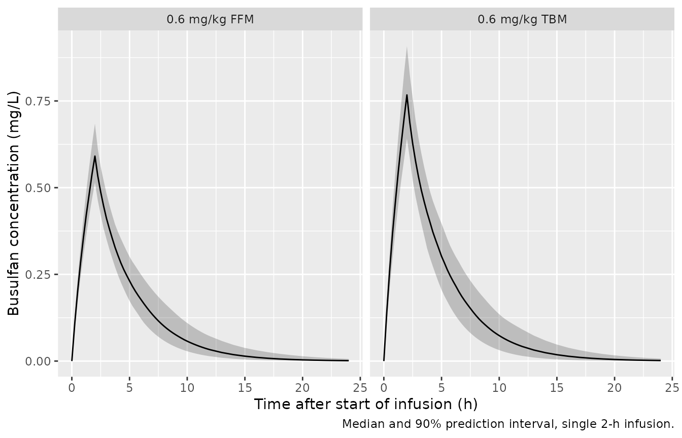
Concentration-time profiles
sim |>
  filter(time <= 24) |>
  group_by(arm, time) |>
  summarise(
    Q05 = quantile(Cc, 0.05), Q50 = median(Cc), Q95 = quantile(Cc, 0.95),
    .groups = "drop"
  ) |>
  ggplot(aes(time, Q50)) +
  geom_ribbon(aes(ymin = Q05, ymax = Q95), alpha = 0.25) +
  geom_line() +
  facet_wrap(~arm) +
  labs(
    x = "Time after start of infusion (h)", y = "Busulfan concentration (mg/L)",
    caption = "Median and 90% prediction interval, single 2-h infusion."
  )
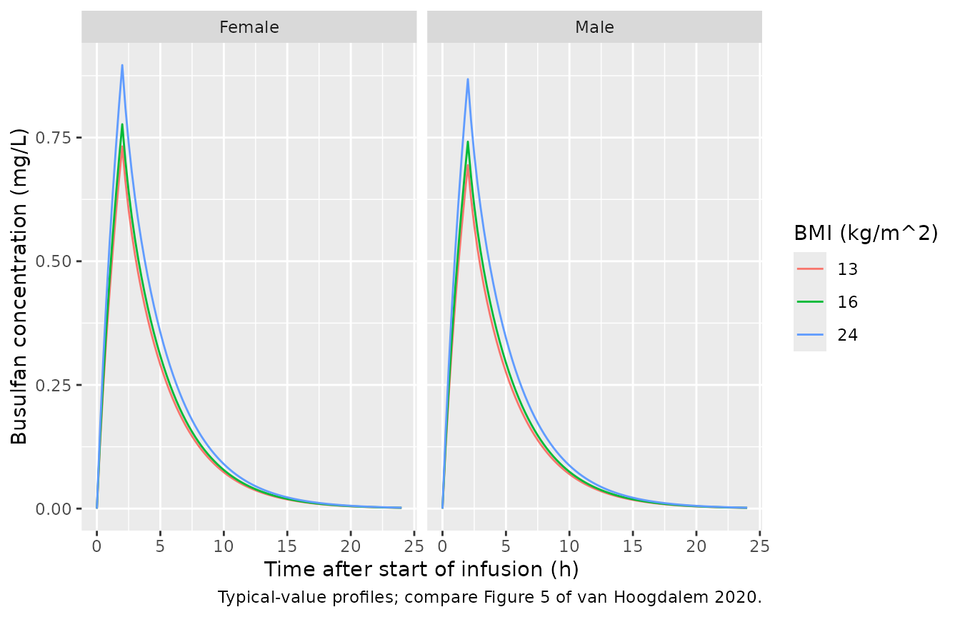
Typical-value profiles for an 8-year-old of 120 cm who is underweight (BMI 13), normal weight (BMI 16) or obese (BMI 24), after a 0.6 mg/kg TBM dose. This mirrors the underweight / normal / obese comparison of Figure 5.
typ <- tidyr::crossing(SEXF = c(0, 1), BMI = c(13, 16, 24)) |>
  mutate(
    id = row_number(), AGE = 8, HT = 120,
    WT = BMI * 1.2^2, FFM = ffm_alsallami(AGE, HT, WT, SEXF)
  )
typ_ev <- bind_rows(
  typ |> mutate(time = 0, amt = 0.6 * WT, evid = 1, cmt = "central", dur = 2),
  tidyr::crossing(typ, time = seq(0, 24, by = 0.25)) |>
    mutate(amt = 0, evid = 0, cmt = "central", dur = 0)
) |> arrange(id, time, desc(evid))

sim_typ <- rxode2::rxSolve(rxode2::zeroRe(mod), events = typ_ev, keep = c("BMI", "SEXF")) |>
  as.data.frame()
#> ℹ parameter labels from comments will be replaced by 'label()'
#> ℹ omega/sigma items treated as zero: 'etalcl', 'etalvc'
#> Warning: multi-subject simulation without without 'omega'

ggplot(sim_typ, aes(time, Cc, colour = factor(BMI))) +
  geom_line() +
  facet_wrap(~ ifelse(SEXF == 1, "Female", "Male")) +
  labs(
    x = "Time after start of infusion (h)", y = "Busulfan concentration (mg/L)",
    colour = "BMI (kg/m^2)",
    caption = "Typical-value profiles; compare Figure 5 of van Hoogdalem 2020."
  )
PKNCA validation and steady-state concentration
sim_nca <- sim |>
  filter(!is.na(Cc)) |>
  select(id, time, Cc, arm)

dose_df <- events |>
  filter(evid == 1) |>
  select(id, time, amt, dur, arm)

conc_obj <- PKNCA::PKNCAconc(sim_nca, Cc ~ time | arm + id)
dose_obj <- PKNCA::PKNCAdose(dose_df, amt ~ time | arm + id, duration = "dur", route = "intravascular")
intervals <- data.frame(start = 0, end = Inf, cmax = TRUE, tmax = TRUE, aucinf.obs = TRUE, half.life = TRUE)
nca_res <- PKNCA::pk.nca(PKNCA::PKNCAdata(conc_obj, dose_obj, intervals = intervals))

nca_wide <- as.data.frame(nca_res) |>
  filter(PPTESTCD %in% c("cmax", "aucinf.obs", "half.life")) |>
  select(id, arm, PPTESTCD, PPORRES) |>
  tidyr::pivot_wider(names_from = PPTESTCD, values_from = PPORRES)

summary(nca_res)
#>  start end           arm   N         cmax              tmax    half.life
#>      0 Inf 0.6 mg/kg FFM 200 0.593 [8.51] 2.00 [2.00, 2.00] 2.55 [0.476]
#>      0 Inf 0.6 mg/kg TBM 200 0.765 [10.8] 2.00 [2.00, 2.00] 2.52 [0.458]
#>   aucinf.obs
#>  2.65 [16.1]
#>  3.39 [17.3]
#>
#> Caption: cmax, aucinf.obs: geometric mean and geometric coefficient of variation; tmax: median and range; half.life: arithmetic mean and standard deviation; N: number of subjects
The NCA AUC is checked against the exact dose / CL of
each simulated subject, which uses the same drawn parameters; the
difference is pure numerical (trapezoid and extrapolation) error, so a
tight bound applies.
indiv <- sim |>
  group_by(id, arm) |>
  summarise(cl = first(cl), FFM = first(FFM), WT = first(WT), BMI = first(BMI),
            obese = first(obese), .groups = "drop") |>
  left_join(dose_df |> select(id, amt), by = "id") |>
  left_join(nca_wide, by = c("id", "arm")) |>
  mutate(
    auc_exact = amt / cl,
    pct_diff = 100 * (aucinf.obs - auc_exact) / auc_exact,
    Css = aucinf.obs / 12
  )
summary(indiv$pct_diff)
#>     Min.  1st Qu.   Median     Mean  3rd Qu.     Max.
#> -0.07654 -0.04498 -0.03693 -0.03789 -0.02862 -0.01337
stopifnot(all(abs(indiv$pct_diff) < 2))
Under FFM-based dosing the typical Css does not depend
on body composition at all: with CL = 12.6 * FFM / 56.1, a
dose of d * FFM gives
Css = d * 56.1 / (12.6 * 12). The typical-value solve
confirms this exactly.
typ_ffm <- cohort |>
  mutate(cl_typ = 12.6 * FFM / 56.1, Css_TBM = 0.6 * WT / (cl_typ * 12), Css_FFM = 0.6 * FFM / (cl_typ * 12))
css_ffm_typ <- 0.6 * 56.1 / (12.6 * 12)
css_ffm_typ
#> [1] 0.222619
stopifnot(all(abs(typ_ffm$Css_FFM - css_ffm_typ) < 1e-12))
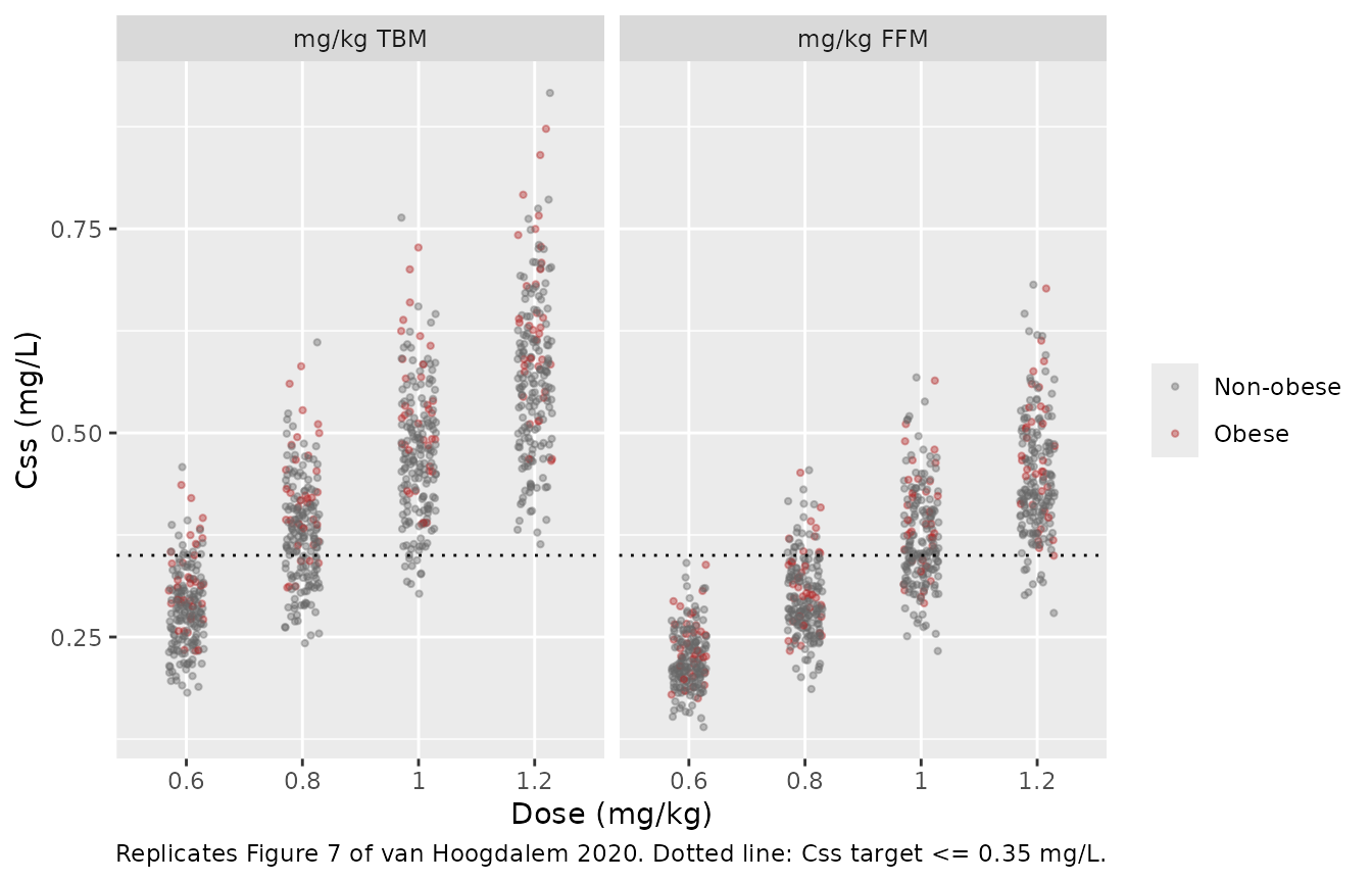
Comparison against published Css (Figure 7 / Results 3.3)
The paper reports the mean and interquartile range of the individual
Bayesian Css estimates of its 29 patients for each
simulated dose (Results 3.3).
published <- tibble::tribble(
  ~basis, ~dose, ~pub_mean, ~pub_q25, ~pub_q75,
  "TBM", 0.6, 0.28, 0.25, 0.30,
  "TBM", 0.8, 0.37, 0.33, 0.41,
  "TBM", 1.0, 0.46, 0.41, 0.51,
  "TBM", 1.2, 0.55, 0.49, 0.61,
  "FFM", 0.6, 0.21, 0.20, 0.23,
  "FFM", 0.8, 0.28, 0.26, 0.30,
  "FFM", 1.0, 0.35, 0.33, 0.38,
  "FFM", 1.2, 0.43, 0.39, 0.45
)

css_scen <- indiv |>
  mutate(basis = ifelse(grepl("TBM", arm), "TBM", "FFM")) |>
  tidyr::crossing(dose = c(0.6, 0.8, 1.0, 1.2)) |>
  mutate(Css_d = Css * dose / 0.6)

css_sum <- css_scen |>
  group_by(basis, dose) |>
  summarise(
    sim_mean = mean(Css_d), sim_q25 = quantile(Css_d, 0.25), sim_q75 = quantile(Css_d, 0.75),
    .groups = "drop"
  ) |>
  left_join(published, by = c("basis", "dose")) |>
  mutate(pct_diff = 100 * (sim_mean - pub_mean) / pub_mean)

css_sum |>
  mutate(
    Simulated = sprintf("%.3f (%.3f-%.3f)", sim_mean, sim_q25, sim_q75),
    Published = sprintf("%.2f (%.2f-%.2f)", pub_mean, pub_q25, pub_q75),
    `Difference (%)` = sprintf("%+.1f", pct_diff)
  ) |>
  select(basis, dose, Simulated, Published, `Difference (%)`) |>
  dplyr::rename("Dose basis" = basis, "Dose (mg/kg)" = dose, "Simulated mean (IQR), mg/L" = Simulated,
                "Published mean (IQR), mg/L" = Published) |>
knitr::kable(caption = "Css after a single dose, tau = 12 h (van Hoogdalem 2020 Results 3.3 / Figure 7).")| Dose basis | Dose (mg/kg) | Simulated mean (IQR), mg/L | Published mean (IQR), mg/L | Difference (%) |
|---|---|---|---|---|
| FFM | 0.6 | 0.224 (0.200-0.247) | 0.21 (0.20-0.23) | +6.7 |
| FFM | 0.8 | 0.299 (0.266-0.329) | 0.28 (0.26-0.30) | +6.7 |
| FFM | 1.0 | 0.373 (0.333-0.412) | 0.35 (0.33-0.38) | +6.7 |
| FFM | 1.2 | 0.448 (0.399-0.494) | 0.43 (0.39-0.45) | +4.2 |
| TBM | 0.6 | 0.287 (0.252-0.315) | 0.28 (0.25-0.30) | +2.4 |
| TBM | 0.8 | 0.382 (0.336-0.420) | 0.37 (0.33-0.41) | +3.4 |
| TBM | 1.0 | 0.478 (0.420-0.525) | 0.46 (0.41-0.51) | +3.9 |
| TBM | 1.2 | 0.574 (0.504-0.630) | 0.55 (0.49-0.61) | +4.3 |
# A cohort mean, not an extreme: a mis-transcribed clearance or reference FFM
# moves every row by tens of percent.
stopifnot(all(abs(css_sum$pct_diff) < 15))
The simulated IQRs are wider than the published ones, and the
FFM-based IQR is only slightly narrower than the TBM-based one. The
published IQRs summarise 29 Bayesian post-hoc estimates, which shrink
toward the population value, whereas the simulation draws the full IIV
on CL (16.2% CV). In the simulation most of the spread in
Css comes from that IIV rather than from body composition.
The part of the spread that body composition causes is removed
completely by FFM dosing, as the closed-form check above shows.
ggplot(css_scen, aes(factor(dose), Css_d, colour = obese)) +
  geom_jitter(width = 0.15, alpha = 0.4, size = 0.8) +
  geom_hline(yintercept = 0.35, linetype = "dotted") +
  facet_wrap(~ factor(basis, levels = c("TBM", "FFM"), labels = c("mg/kg TBM", "mg/kg FFM"))) +
  scale_colour_manual(values = c(`FALSE` = "grey40", `TRUE` = "firebrick"), labels = c("Non-obese", "Obese")) +
  labs(
    x = "Dose (mg/kg)", y = "Css (mg/L)", colour = NULL,
    caption = "Replicates Figure 7 of van Hoogdalem 2020. Dotted line: Css target <= 0.35 mg/L."
  )
Css versus BMI (Figure 6)
Under TBM dosing Css rises with BMI; under FFM dosing it
is flat. The paper reports a significant positive slope for 0.6 mg/kg
TBM (P < 0.001) and no slope for 0.6 or 0.8 mg/kg FFM (P = 0.57 and
0.54).
indiv_06 <- css_scen |> filter(dose == 0.6)
ggplot(indiv_06, aes(BMI, Css_d)) +
  geom_point(alpha = 0.5) +
  geom_smooth(method = "lm", formula = y ~ x) +
  facet_wrap(~ factor(basis, levels = c("TBM", "FFM"), labels = c("0.6 mg/kg TBM", "0.6 mg/kg FFM"))) +
  labs(x = "BMI (kg/m^2)", y = "Css (mg/L)", caption = "Compare Figure 6B-C of van Hoogdalem 2020.")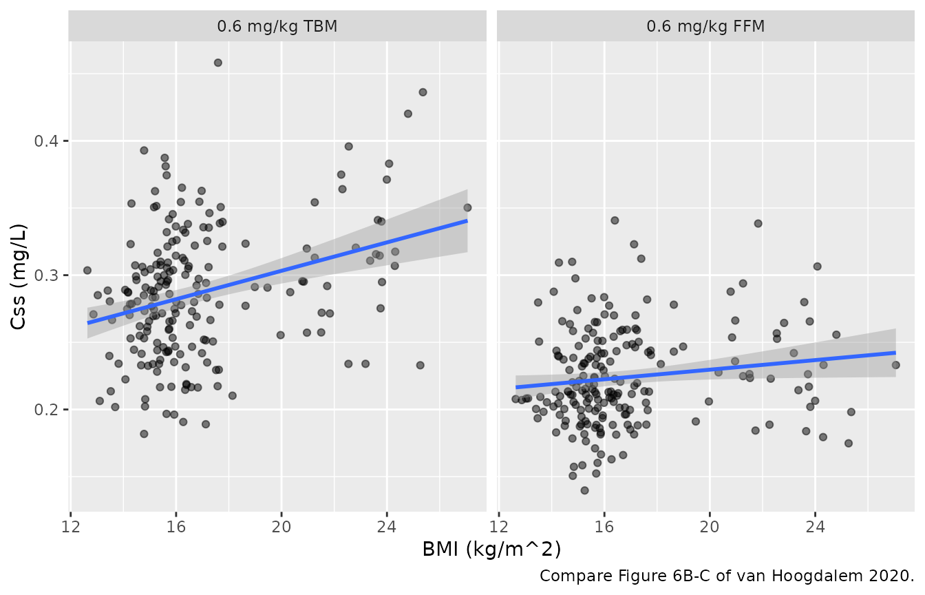
# The typical-value relation is deterministic: under TBM dosing Css rises
# strictly with WT/FFM, which rises with BMI at fixed age, sex and height.
stopifnot(cor(typ_ffm$BMI, typ_ffm$Css_TBM, method = "spearman") > 0.5)
obese_tbm <- indiv_06 |>
  filter(basis == "TBM") |>
  group_by(obese) |>
  summarise(mean_Css = mean(Css_d), sd_Css = sd(Css_d), n = n())
knitr::kable(obese_tbm, digits = 3,
caption = "0.6 mg/kg TBM: published non-obese 0.265 (SD 0.040) vs obese 0.345 (SD 0.074) mg/L.")| obese | mean_Css | sd_Css | n |
|---|---|---|---|
| FALSE | 0.281 | 0.047 | 164 |
| TRUE | 0.314 | 0.051 | 36 |
Assumptions and deviations
-
IIV scale. Table 2 reports IIV as CV% without
stating the conversion; the variances use
omega^2 = log(CV^2 + 1). At CVs of 12-16% this differs fromCV^2by under 2%. -
Dosing interval. Equation 9 uses tau; the 12-hour
interval of the source trial (Methods 2.4) is used. It reproduces the
published 0.6 mg/kg TBM mean
Css(0.28 mg/L) for a typical patient of the median size. - IIV on Q and V2 was fixed to 0 in the source and is omitted.
- FFM as a data column. The model takes FFM directly; the vignette computes it with Equations 3-4 (Al-Sallami paediatric form). The authors note the equation was derived in subjects aged 3-29 years.
-
Virtual cohort. Individual demographics are not
available. The height, BMI and obesity proportions are approximations of
Table 1 and Figure 1, so TBM-based
Cssvalues (which depend on each patient’s WT/FFM ratio) are only expected to agree in location, not in spread. The published medians of height (120.6 cm) and BMI (16.0 kg/m^2) imply a heavier median patient than the published median weight (19.9 kg), so the virtual cohort’s median weight (about 25 kg) is higher than Table 1’s. -
Published Css are Bayesian post-hoc estimates in 29
patients (Methods 2.4, MwPharm++), not simulations from the population
model. The simulated FFM-based means are about 5-7% above the published
means; the typical-value prediction
0.6 * 56.1 / (12.6 * 12)= 0.223 mg/L is itself 6% above the published 0.21 mg/L, so the offset is a property of the 29 observed patients’ individual clearances rather than of the model transcription. - Obese classification in the virtual cohort is a flag on the sampled BMI multiplier, not the age- and sex-specific Cole cut-offs used in the paper.