Ibrutinib posology optimization in CLL (Ibrahim 2025)
Source:vignettes/articles/Ibrahim_2025_ibrutinib.Rmd
Ibrahim_2025_ibrutinib.RmdModels and source
Ibrahim 2025 re-estimates and extends the semi-mechanistic ibrutinib
framework of Ibrahim 2023, pooling the phase Ib/II PCYC-1102 and phase
III PCYC-1115 studies (n = 246). Two models were fitted, in two separate
nlmixr runs, and a third configuration was calibrated for
the ibrutinib + venetoclax combination. They are packaged as three model
files.
| Model file | Endpoint(s) | Source |
|---|---|---|
Ibrahim_2025_ibrutinib_cll |
leukocyte count, lymphocyte count, SPD, spleen volume | Data S1 run8634_eff; eq. 2-5; Table 1 |
Ibrahim_2025_ibrutinib_bp |
systolic and diastolic blood pressure | Data S1 run6023_bp; Table 2 |
Ibrahim_2025_ibrutinib_venetoclax |
as _cll, plus peripheral-blood MRD |
as _cll, plus Table S2 |
- Citation: Ibrahim EIK, Friberg LE. Optimizing Ibrutinib Posology in
Chronic Lymphocytic Leukemia Using a Semi-Mechanistic Pharmacometric
Framework. CPT Pharmacometrics Syst Pharmacol. 2025;14(12):2186-2197. doi:10.1002/psp4.70124.
Open Access under CC BY-NC. Structural equations transcribed from the
authors’ own RxODE control stream (Data S1, PSP-2025-0220-s02.docx,
run8634_eff); observation equations from main-text equations 2-5; parameter values from Table 1. Model structure inherited from Ibrahim EIK, Karlsson MO, Friberg LE. CPT Pharmacometrics Syst Pharmacol. 2023;12(9):1305-1318. doi:10.1002/psp4.13010; see modellib(‘Ibrahim_2023_ibrutinib_leukocyte_spd’). - Article: https://doi.org/10.1002/psp4.70124
- Supplement (Table S1, Table S2, figure captions, and the authors’
own RxODE control streams): Data S1,
psp470124-sup-0001-DataS1.zip, via https://doi.org/10.1002/psp4.70124
The structural equations in all three files are transcribed from the
authors’ own RxODE control streams, published verbatim in Data S1
(PSP-2025-0220-s02.docx). The parameter values come from
Tables 1, 2 and S2 – unlike the 2023 predecessor, Data S1 supplies the
model code but not the fitted THETA vector, so every value is
the rounded, back-transformed published point estimate rather than a
higher-precision control-stream number.
mCll <- rxode2::rxode(modellib("Ibrahim_2025_ibrutinib_cll"))
#> ℹ parameter labels from comments will be replaced by 'label()'
mBp  <- rxode2::rxode(modellib("Ibrahim_2025_ibrutinib_bp"))
#> ℹ parameter labels from comments will be replaced by 'label()'
mVen <- rxode2::rxode(modellib("Ibrahim_2025_ibrutinib_venetoclax"))
#> ℹ parameter labels from comments will be replaced by 'label()'
Population
The analysis pooled 246 patients with chronic lymphocytic leukemia from two Janssen studies made available through the Yale University Open Data Access (YODA) Project 2020-4386: the non-randomized open-label phase Ib/II PCYC-1102 (n = 120 with ibrutinib concentrations plus leukocyte count and SPD; ibrutinib 420 mg/day, n = 94, or 840 mg/day, n = 38) and the randomized open-label phase III PCYC-1115 (n = 126 with ibrutinib concentrations plus leukocyte or lymphocyte count and SPD or spleen volume; ibrutinib 420 mg/day). Mean baseline age was 70 (SD 8.9) years; 151 patients (61%) were treatment-naive (TN) and 95 (39%) were relapsed/refractory (R/R) (Table S1).
Table S1 of the 2025 paper reports only age and CLL
group for the pooled population, so the population metadata
of these three files deliberately omits weight, sex and race rather than
carrying them over from the 2023 predecessor, whose population is a
strict subset.
str(rxode2::rxode(modellib("Ibrahim_2025_ibrutinib_cll"))$population)
#> ℹ parameter labels from comments will be replaced by 'label()'
#> List of 8
#>  $ species      : chr "human"
#>  $ n_subjects   : int 246
#>  $ n_studies    : int 2
#>  $ age_range    : chr "mean 70 (SD 8.9) years"
#>  $ disease_state: chr "Chronic lymphocytic leukemia (CLL); 151 (61%) treatment-naive, 95 (39%) relapsed/refractory"
#>  $ dose_range   : chr "ibrutinib 420 mg once daily (n = 94) or 840 mg once daily (n = 38) in PCYC-1102; 420 mg once daily in PCYC-1115"
#>  $ regions      : chr "United States and international (PCYC-1102 phase Ib/II; PCYC-1115 phase III)"
#>  $ notes        : chr "Baseline demographics from Ibrahim 2025 Table S1 (Data S1, PSP-2025-0220-s01.docx), which reports only age and "| __truncated__
Source trace
The per-parameter origin is recorded as an in-file comment next to
every ini() entry. The table below collects the structural
equations.
Structural equations
| Equation | Source |
|---|---|
d/dt(pbtk) = kin*(1-effauc) - kout*pbtk |
Data S1 run8634_eff, ODE block |
d/dt(cll_subpop1), d/dt(cll_subpop2)
(proliferation - detachment) |
Data S1 run8634_eff (rln_spd,
rln_spdq) |
d/dt(cll_subpop3) (proliferation + detachment influx +
homing influx - redistribution - ibrutinib apoptosis) |
Data S1 run8634_eff (ln_spd) |
d/dt(cll_bld) (redistribution influx - homing efflux -
death) |
Data S1 run8634_eff (bld_tcll) |
SPD = (subpop1+subpop2+subpop3)*(SPDbaseline/CLLtiss,baseline) + SPDnrm |
main text eq. 2 |
Spleen = (subpop1+subpop2+subpop3)*(SPLEENbaseline/CLLtiss,baseline) + SPLEENnrm |
main text eq. 3 |
Leukocyte = (subpop4 + LEUKnrm)/Vbld |
main text eq. 4 |
Lymphocyte = (subpop4 + f_lymphocyte*LEUKnrm)/Vbld |
main text eq. 5 |
kdist = (kh + kd,bld)*(CLLbld,baseline/(f2*CLLtiss,baseline)) |
Data S1 run8634_eff (krd) |
kdtch = kp |
Table 1 footnote c |
BP: d/dt(transit) = kin*(1+eff) - ktr*transit;
d/dt(bp) = ktr*transit - kout*bp;
kout = ktr = 2/MTT
|
Data S1 run6023_bp
|
Venetoclax tissue kill kd,bld*Emax,i*C/(EC50,tiss+C);
blood kd,bld*(1+Emax,4*C/(EC50,bld+C))
|
Table S2 footnote a |
Units
Every rate constant is per day and every CLL state
is a cell count in units of 10^9 cells, so each ODE term carries
(1/day) * 10^9 cells = 10^9 cells/day, matching the
left-hand side. Because the 2025 parameterisation keeps all four CLL
subpopulations on the cell-count scale (the 2023 predecessor carried the
tissue pools on the SPD scale), no cell-to-SPD conversion factor appears
inside the ODEs at all – the conversion
SPDbaseline/CLLtiss,baseline
(cm^2 / 10^9 cells) is applied once, at the observation
step, giving cm^2. The same holds for spleen volume with
cc / 10^9 cells. Vbld (L) converts the
peripheral-blood cell number to a count per litre. Blood pressure is in
mmHg and ktr = kout = 2/MTT is per day.
Two parameters in Table 1 are tabulated per month
while the model integrates in days (kout,pBtk,
kh, kd,bld and kd,tiss are all
tabulated per day and are used directly against t). Both
are converted with 30 days per month; see Assumptions and deviations.
tibble::tibble(
  Parameter = c("kp", "lambda_dec"),
  `Table 1 (per month)` = c(0.124, 0.0230),
  `Model (per day)` = signif(c(0.124, 0.0230) / 30, 4),
  `Ibrahim 2023 (per day)` = c(0.00416, 0.000911)
) |>
  knitr::kable(
    caption = "Month-to-day conversion, cross-checked against the 2023 predecessor."
)| Parameter | Table 1 (per month) | Model (per day) | Ibrahim 2023 (per day) |
|---|---|---|---|
| kp | 0.124 | 0.0041330 | 0.004160 |
| lambda_dec | 0.023 | 0.0007667 | 0.000911 |
Structural identities implied by the published covariate effects
Several of the paper’s headline numerical claims are exact algebraic consequences of Table 1, so they are strict tests of the transcription rather than approximate comparisons. Each is asserted below; a wrong sign, a misread multiplier or a transposed row would break them.
iniCll <- mCll$iniDf
th <- function(nm) iniCll$est[match(nm, iniCll$name)]

kout_tn <- exp(th("lkout_pbtk"))
kout_rr <- exp(th("lkout_pbtk") + th("e_rr_kout_pbtk"))
kdb_tn  <- exp(th("lkd_bld"))
kdb_rr  <- exp(th("lkd_bld") + th("e_rr_kd_bld"))

# 1. "a 76% longer phospho-Btk half-life ... in TN versus R/R patients"
pbtk_hl_ratio <- (log(2) / kout_tn) / (log(2) / kout_rr)

# 2. "a 43% shorter peripheral CLL cell half-life in TN versus R/R"
cll_hl_tn <- log(2) / kdb_tn
cll_hl_rr <- log(2) / kdb_rr
cll_hl_shortening <- 1 - cll_hl_tn / cll_hl_rr

# 3. "TN patients ... 3.91- and 1.87-fold higher baseline CLL cell count in
#    peripheral blood and LEUKnrm, respectively, compared to R/R patients"
cllbld_ratio <- exp(th("lrbase_cllbld_tn")) / exp(th("lrbase_cllbld_rr"))
leuknrm_ratio <- exp(th("lleuknrm_tn")) / exp(th("lleuknrm_rr"))

# 4. "A 47% lower normal leukocyte count in R/R patients compared to TN"
leuknrm_drop <- 1 - exp(th("lleuknrm_rr")) / exp(th("lleuknrm_tn"))

# 5. "The 58% higher SPD in R/R patients compared to TN patients"
spd_ratio <- exp(th("e_rr_rbase_spd"))

stopifnot(
  isTRUE(all.equal(pbtk_hl_ratio,     1.76,  tolerance = 1e-3)),
  isTRUE(all.equal(cll_hl_shortening, 0.429, tolerance = 2e-3)),
  isTRUE(all.equal(cllbld_ratio,      3.91,  tolerance = 2e-3)),
  isTRUE(all.equal(leuknrm_ratio,     1.87,  tolerance = 3e-3)),
  isTRUE(all.equal(leuknrm_drop,      0.466, tolerance = 5e-3)),
  isTRUE(all.equal(spd_ratio,         1.58,  tolerance = 1e-6))
)

tibble::tibble(
  Claim = c(
    "pBtk half-life ratio, TN / R/R",
    "peripheral CLL half-life shortening in TN",
    "baseline blood CLL count ratio, TN / R/R",
    "normal leukocyte count ratio, TN / R/R",
    "normal leukocyte count reduction in R/R",
    "baseline SPD ratio, R/R / TN"
  ),
  Published = c("1.76 (76% longer)", "43% shorter", "3.91-fold",
                "1.87-fold", "47% lower", "1.58 (58% higher)"),
  Model = c(
    sprintf("%.3f", pbtk_hl_ratio), sprintf("%.1f%%", 100 * cll_hl_shortening),
    sprintf("%.3f", cllbld_ratio), sprintf("%.3f", leuknrm_ratio),
    sprintf("%.1f%%", 100 * leuknrm_drop), sprintf("%.3f", spd_ratio)
  )
) |>
knitr::kable(caption = "Exact identities implied by Table 1.")| Claim | Published | Model |
|---|---|---|
| pBtk half-life ratio, TN / R/R | 1.76 (76% longer) | 1.760 |
| peripheral CLL half-life shortening in TN | 43% shorter | 42.9% |
| baseline blood CLL count ratio, TN / R/R | 3.91-fold | 3.910 |
| normal leukocyte count ratio, TN / R/R | 1.87-fold | 1.874 |
| normal leukocyte count reduction in R/R | 47% lower | 46.6% |
| baseline SPD ratio, R/R / TN | 1.58 (58% higher) | 1.580 |
The pBtk half-lives themselves are 1.32 days (TN) and 0.75 days (R/R); the peripheral CLL cell half-lives are 45 days (TN) and 79 days (R/R).
The exposure input
Both fitted models are driven by the daily AUC(0-24) of ibrutinib,
which the authors computed from the individual plasma concentrations
using the two-compartment population PK model of Marostica et
al. (Cancer Chemother Pharmacol. 2015;75(1):111-121). That upstream PK
model is not part of nlmixr2lib and the
paper tabulates no AUC values, so the exposure per dose level has to be
reconstructed. Two independent routes are available and they agree
closely.
Route 1 (used here) – the upstream PK paper.
Marostica 2015 reports an apparent oral plasma clearance of
approximately 1000 L/h and states that “PK parameters were not dependent
on dose, study, or clinical indication”, i.e. exposure is
dose-proportional. At steady state
AUC(0-24) = Dose / (CL/F), so 420 mg/day gives
420 mg / 1000 L/h = 0.42 mg*h/L = 420 h*ng/mL, i.e. **1.0
h*ng/mL per mg**.
Route 2 (cross-check) – inverting the 2023 paper’s reported
Btk occupancy. The 2023 companion paper reports median
steady-state Btk occupancy of 92.7%, 89.4% and 80.8% at 420, 280 and 140
mg/day. At steady state the pBtk turnover model collapses to
pBtk = 1 - EFF, so
AUC = IAUC50 * occ / (1 - occ) with the 2023
IAUC50 of 34.1 hng/mL. That inversion yields 1.032,
1.028 and 1.026 hng/mL per mg.
auc_per_mg_marostica <- 1000 / 1000        # (mg/day) / (L/h) -> h*ng/mL per mg
iauc50_2023 <- 34.1
occ_2023 <- c(`420` = 0.927, `280` = 0.894, `140` = 0.808)
auc_per_mg_2023 <- iauc50_2023 * occ_2023 / (1 - occ_2023) /
  as.numeric(names(occ_2023))

tibble::tibble(
  `Dose (mg/day)` = as.numeric(names(occ_2023)),
  `AUC per mg, from Marostica CL/F` = auc_per_mg_marostica,
  `AUC per mg, from 2023 occupancy` = signif(auc_per_mg_2023, 4),
  `Relative difference` = sprintf("%.1f%%", 100 * (auc_per_mg_2023 - auc_per_mg_marostica) / auc_per_mg_marostica)
) |>
knitr::kable(caption = "Two independent reconstructions of the ibrutinib exposure input.")| Dose (mg/day) | AUC per mg, from Marostica CL/F | AUC per mg, from 2023 occupancy | Relative difference |
|---|---|---|---|
| 420 | 1 | 1.031 | 3.1% |
| 280 | 1 | 1.027 | 2.7% |
| 140 | 1 | 1.025 | 2.5% |
stopifnot(all(abs(auc_per_mg_2023 - auc_per_mg_marostica) < 0.05))

aucFor <- function(dose_mg) auc_per_mg_marostica * dose_mg
The two routes agree to within 3.2%, which is a meaningful check:
they share no inputs beyond the drug itself (one is an apparent
clearance from a separate popPK publication, the other is a
pharmacodynamic occupancy inverted through a different paper’s
IAUC50). The resulting AUC values are nonetheless
derived, not published – see Assumptions
and deviations.
With IAUC50 = 28.4 h*ng/mL (Table 1) these exposures
imply the following steady-state Btk occupancies, which bracket the 2023
reported values:
iauc50_2025 <- exp(th("liauc50_pbtk"))
tibble::tibble(
  `Dose (mg/day)` = c(420, 280, 140),
  `AUC(0-24) (h*ng/mL)` = aucFor(c(420, 280, 140)),
  `Btk occupancy (%)` = sprintf("%.1f", 100 * aucFor(c(420, 280, 140)) /
                                  (iauc50_2025 + aucFor(c(420, 280, 140)))),
  `Ibrahim 2023 reported (%)` = c(92.7, 89.4, 80.8)
) |>
knitr::kable(caption = "Implied steady-state Btk occupancy by ibrutinib dose level.")| Dose (mg/day) | AUC(0-24) (h*ng/mL) | Btk occupancy (%) | Ibrahim 2023 reported (%) |
|---|---|---|---|
| 420 | 420 | 93.7 | 92.7 |
| 280 | 280 | 90.8 | 89.4 |
| 140 | 140 | 83.1 | 80.8 |
The CLL model
Drug-free behaviour and the pseudo-steady-state construction
With AUC_IBRU = 0 there is no drug effect, so
pbtk must sit exactly at its baseline of 1 and the
peripheral-blood pool must be in flux balance – which is precisely what
the kdist definition enforces. At t = 0 and
zero exposure the blood-pool influx is
kdist * cll_subpop3(0)
  = (kh + kd,bld) * (CLLbld,0 / (f2 * CLLtiss,0)) * (f2 * CLLtiss,0)
  = (kh + kd,bld) * CLLbld,0
which cancels exactly against the efflux
(kh + kd,bld) * cll_bld(0). The tissue pool, by contrast,
is deliberately not at steady state – untreated CLL grows.
typCll <- rxode2::zeroRe(mCll, which = c("omega", "sigma"))

obsGrid <- function(times, cmt = "cll_bld") {
  tibble::tibble(time = times, evid = 0L, cmt = cmt, dvid = 1L)
}

evFree <- obsGrid(seq(0, 730, by = 7)) |>
  mutate(AUC_IBRU = 0, LINE_1L = 1)
simFree <- rxode2::rxSolve(typCll$simulationModel, evFree,
                           useLinCmt = FALSE, returnType = "data.frame")
#> ℹ omega/sigma items treated as zero: 'etalkout_pbtk', 'etalrbase_cllbld_tn', 'etalrbase_cllbld_rr', 'etalogit_flymphocyte', 'etalrbase_clltiss', 'etalrbase_spleen', 'etalleuknrm_tn', 'etalleuknrm_rr', 'etalspleennrm', 'etalogit_f1', 'etalogit_f2', 'etalkp', 'etalkh', 'etaliauc50_pbtk', 'etalkd_tiss', 'etallambda_dec', 'etalspdnrm_rad', 'etalrbase_spd', 'etalspdnrm'

row0 <- simFree[simFree$time == 0, ]
influx <- row0$kdist * row0$cll_subpop3
efflux <- (row0$kh + row0$kd_bld) * row0$cll_bld

stopifnot(
  isTRUE(all.equal(range(simFree$pbtk), c(1, 1), tolerance = 1e-8)),
  isTRUE(all.equal(influx, efflux, tolerance = 1e-8)),
  # untreated disease must grow on every tissue output
  dplyr::last(simFree$tumorSpd)     > simFree$tumorSpd[1],
  dplyr::last(simFree$spleenVolume) > simFree$spleenVolume[1]
)

tibble::tibble(
  Check = c("pBtk range without drug", "blood-pool influx at t=0",
            "blood-pool efflux at t=0"),
  Value = c(paste(signif(range(simFree$pbtk), 8), collapse = " to "),
            signif(influx, 6), signif(efflux, 6))
) |>
knitr::kable(caption = "Drug-free consistency of the CLL model.")| Check | Value |
|---|---|
| pBtk range without drug | 1 to 1 |
| blood-pool influx at t=0 | 122.366 |
| blood-pool efflux at t=0 | 122.366 |
Baseline observations reproduce the published typical values
At t = 0 each of the four outputs must equal its Table 1
construction exactly. This checks equations 2-5 and the initial
conditions simultaneously, in both patient groups.
baselineFor <- function(line1l) {
  ev <- obsGrid(0) |> mutate(AUC_IBRU = 0, LINE_1L = line1l)
  rxode2::rxSolve(typCll$simulationModel, ev,
                  useLinCmt = FALSE, returnType = "data.frame")
}
bTn <- baselineFor(1L)
#> ℹ omega/sigma items treated as zero: 'etalkout_pbtk', 'etalrbase_cllbld_tn', 'etalrbase_cllbld_rr', 'etalogit_flymphocyte', 'etalrbase_clltiss', 'etalrbase_spleen', 'etalleuknrm_tn', 'etalleuknrm_rr', 'etalspleennrm', 'etalogit_f1', 'etalogit_f2', 'etalkp', 'etalkh', 'etaliauc50_pbtk', 'etalkd_tiss', 'etallambda_dec', 'etalspdnrm_rad', 'etalrbase_spd', 'etalspdnrm'
bRr <- baselineFor(0L)
#> ℹ omega/sigma items treated as zero: 'etalkout_pbtk', 'etalrbase_cllbld_tn', 'etalrbase_cllbld_rr', 'etalogit_flymphocyte', 'etalrbase_clltiss', 'etalrbase_spleen', 'etalleuknrm_tn', 'etalleuknrm_rr', 'etalspleennrm', 'etalogit_f1', 'etalogit_f2', 'etalkp', 'etalkh', 'etaliauc50_pbtk', 'etalkd_tiss', 'etallambda_dec', 'etalspdnrm_rad', 'etalrbase_spd', 'etalspdnrm'

# Expected values built directly from the Table 1 rows.
expTn <- c(
  leukocyte    = (208 + 37.3) / 5,
  lymphocyte   = (208 + 37.3 * 0.310) / 5,
  tumorSpd     = 24.3 + 2.70,
  spleenVolume = 314 + 252
)
expRr <- c(
  leukocyte    = (53.2 + 19.9) / 5,
  lymphocyte   = (53.2 + 19.9 * 0.310) / 5,
  tumorSpd     = 24.3 * 1.58 + 2.70,
  spleenVolume = 314 + 252
)
gotTn <- c(bTn$leukocyte, bTn$lymphocyte, bTn$tumorSpd, bTn$spleenVolume)
gotRr <- c(bRr$leukocyte, bRr$lymphocyte, bRr$tumorSpd, bRr$spleenVolume)

stopifnot(
  isTRUE(all.equal(unname(gotTn), unname(expTn), tolerance = 1e-6)),
  isTRUE(all.equal(unname(gotRr), unname(expRr), tolerance = 1e-6))
)

tibble::tibble(
  Output = c("leukocyte (10^9/L)", "lymphocyte (10^9/L)",
             "SPD (cm^2)", "spleen volume (cc)"),
  `TN, Table 1` = signif(unname(expTn), 5),
  `TN, model`   = signif(gotTn, 5),
  `R/R, Table 1` = signif(unname(expRr), 5),
  `R/R, model`   = signif(gotRr, 5)
) |>
knitr::kable(caption = "Baseline outputs (eq. 2-5) versus their Table 1 construction.")| Output | TN, Table 1 | TN, model | R/R, Table 1 | R/R, model |
|---|---|---|---|---|
| leukocyte (10^9/L) | 49.060 | 49.060 | 14.620 | 14.620 |
| lymphocyte (10^9/L) | 43.913 | 43.913 | 11.874 | 11.874 |
| SPD (cm^2) | 27.000 | 27.000 | 41.094 | 41.094 |
| spleen volume (cc) | 566.000 | 566.000 | 566.000 | 566.000 |
Note that the tissue baselines are SPDbaseline + SPDnrm,
so the whole tissue compartment is scaled by
SPDbaseline / CLLtiss,baseline – the R/R baseline SPD is
1.58-fold higher while the spleen baseline is shared, which is exactly
the covariate structure Table 1 reports.
Treatment-related lymphocytosis
The clinical signature of ibrutinib is a transient rise in
circulating lymphocytes: blocking homing (eff_home) and
accelerating detachment (eff_dtch1, eff_dtch2)
flushes CLL cells out of the lymph nodes into blood before they are
cleared. Lymph-node burden falls at the same time. The model must
reproduce both limbs at once, and the paper notes the lymphocytosis
“typically resolves within 8 months”.
evTrt <- obsGrid(seq(0, 730, by = 7)) |>
  mutate(AUC_IBRU = aucFor(420), LINE_1L = 1)
simTrt <- rxode2::rxSolve(typCll$simulationModel, evTrt,
                          useLinCmt = FALSE, returnType = "data.frame")
#> ℹ omega/sigma items treated as zero: 'etalkout_pbtk', 'etalrbase_cllbld_tn', 'etalrbase_cllbld_rr', 'etalogit_flymphocyte', 'etalrbase_clltiss', 'etalrbase_spleen', 'etalleuknrm_tn', 'etalleuknrm_rr', 'etalspleennrm', 'etalogit_f1', 'etalogit_f2', 'etalkp', 'etalkh', 'etaliauc50_pbtk', 'etalkd_tiss', 'etallambda_dec', 'etalspdnrm_rad', 'etalrbase_spd', 'etalspdnrm'

peakIdx <- which.max(simTrt$lymphocyte)
peakDay <- simTrt$time[peakIdx]
peakFold <- simTrt$lymphocyte[peakIdx] / simTrt$lymphocyte[1]
# day at which lymphocytes fall back through their baseline
resolvedDay <- simTrt$time[which(simTrt$time > peakDay &
                                   simTrt$lymphocyte <= simTrt$lymphocyte[1])[1]]

stopifnot(
  peakFold > 1,                       # lymphocytosis occurs
  peakDay > 0 && peakDay < 120,       # it is early
  !is.na(resolvedDay),                # and it resolves
  resolvedDay < 365,
  # SPD falls monotonically over the first year while blood counts rise
  dplyr::last(simTrt$tumorSpd[simTrt$time <= 365]) < simTrt$tumorSpd[1]
)

tibble::tibble(
  Quantity = c("peak lymphocyte day", "peak fold-rise over baseline",
               "day lymphocytes return to baseline",
               "SPD at 1 year, fraction of baseline"),
  Value = c(peakDay, signif(peakFold, 3), resolvedDay,
            signif(simTrt$tumorSpd[simTrt$time == 364] / simTrt$tumorSpd[1], 3))
) |>
knitr::kable(caption = "Treatment-related lymphocytosis, typical treatment-naive patient at 420 mg/day.")| Quantity | Value |
|---|---|
| peak lymphocyte day | 21.000 |
| peak fold-rise over baseline | 2.770 |
| day lymphocytes return to baseline | 91.000 |
| SPD at 1 year, fraction of baseline | 0.168 |
simTrt |>
  select(time, lymphocyte, tumorSpd, spleenVolume) |>
  pivot_longer(-time) |>
  mutate(name = factor(name,
                       levels = c("lymphocyte", "tumorSpd", "spleenVolume"),
                       labels = c("Lymphocytes (10^9/L)", "SPD (cm^2)",
                                  "Spleen volume (cc)"))) |>
  ggplot(aes(time, value)) +
  geom_line() +
  facet_wrap(~name, scales = "free_y") +
  labs(x = "Days since ibrutinib start", y = NULL,
       title = "Typical treatment-naive patient, ibrutinib 420 mg/day",
       caption = "Redistribution lymphocytosis with simultaneous nodal and splenic response.")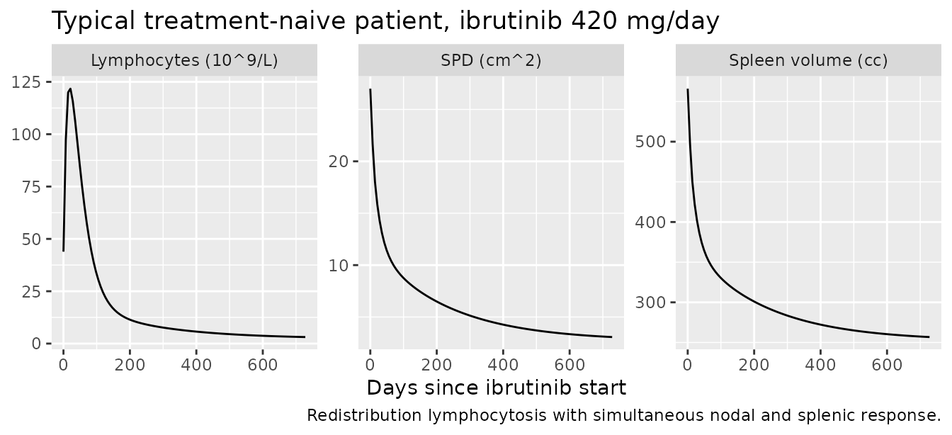
Response rates at two years by dose level
The paper reports that standard 420 mg/day dosing gives the highest
proportion of responders, “averaging 87% and 62% for TN and R/R
patients, respectively, at 2 years” (Results 3.3, Figure S3). Response
is defined as a relative change from baseline of <= -50%
in both SPD and lymphocyte count.
set.seed(20250819)
nPerArm <- 200L

makeArm <- function(n, line1l, dose_mg, label, id_offset) {
  tidyr::crossing(
    tibble::tibble(id = id_offset + seq_len(n), LINE_1L = line1l,
                   arm = label),
    obsGrid(c(0, seq(28, 730, by = 28)))
  ) |>
    mutate(AUC_IBRU = aucFor(dose_mg)) |>
    arrange(id, time)
}

evResp <- bind_rows(
  makeArm(nPerArm, 1L, 420, "TN, 420 mg/day",  id_offset = 0L),
  makeArm(nPerArm, 0L, 420, "R/R, 420 mg/day", id_offset = 1000L)
)
stopifnot(!anyDuplicated(unique(evResp[, c("id", "time", "evid")])))

simResp <- rxode2::rxSolve(mCll, evResp, keep = c("arm", "LINE_1L"),
                           useLinCmt = FALSE, returnType = "data.frame")
# Guard: confirm between-subject variability was actually sampled.
stopifnot(dplyr::n_distinct(simResp$cllbld0) > 1)

responders <- simResp |>
  group_by(arm, id) |>
  arrange(time, .by_group = TRUE) |>
  summarise(
    spdChange  = dplyr::last(tumorSpd) / dplyr::first(tumorSpd) - 1,
    lymChange  = dplyr::last(lymphocyte) / dplyr::first(lymphocyte) - 1,
    .groups = "drop"
  ) |>
  mutate(responder = spdChange <= -0.5 & lymChange <= -0.5)

respSummary <- responders |>
  group_by(arm) |>
  summarise(`Responders at 2 years (%)` = 100 * mean(responder), .groups = "drop") |>
  mutate(`Published (%)` = c(62, 87)[match(arm, c("R/R, 420 mg/day", "TN, 420 mg/day"))])

respSummary |>
  mutate(`Responders at 2 years (%)` = round(`Responders at 2 years (%)`, 1)) |>
knitr::kable(caption = "Simulated versus published two-year response rates (Ibrahim 2025 Results 3.3).")| arm | Responders at 2 years (%) | Published (%) |
|---|---|---|
| R/R, 420 mg/day | 61.5 | 62 |
| TN, 420 mg/day | 92.5 | 87 |
# The published ordering (TN responds better than R/R) is a structural
# consequence of the covariate model and must hold.
tnRate <- respSummary$`Responders at 2 years (%)`[respSummary$arm == "TN, 420 mg/day"]
rrRate <- respSummary$`Responders at 2 years (%)`[respSummary$arm == "R/R, 420 mg/day"]
stopifnot(tnRate > rrRate)
The R/R arm lands on the published value almost exactly (61.5% simulated versus 62% published). The TN arm is 5.5 percentage points high (92.5% versus 87%). Two known contributions account for that direction of error: the paper classified responders from observed measurements and therefore included residual error, which scatters patients across the -50% boundary and – because the TN arm sits well past the threshold – can only move the TN rate down; and at 200 patients per arm the Monte Carlo standard error is about 2 percentage points. No parameter was adjusted to improve the agreement.
Dose de-escalation
The paper’s central clinical claim is that reduced doses retain
efficacy. With IAUC50 = 28.4 h*ng/mL the exposure-response
curve is already near saturation at 420 mg/day, so dropping to 140
mg/day costs little Btk inhibition.
# Each dose arm needs its own id: rxSolve keys subjects on `id`, so arms sharing
# an id silently collapse into one interleaved subject.
doseLevels <- c(420, 280, 140)
evDose <- bind_rows(lapply(seq_along(doseLevels), function(i) {
  d <- doseLevels[i]
  obsGrid(seq(0, 730, by = 14)) |>
    mutate(id = i, AUC_IBRU = aucFor(d), LINE_1L = 1, doseLabel = paste0(d, " mg/day"))
})) |>
  arrange(id, time)
stopifnot(!anyDuplicated(unique(evDose[, c("id", "time", "evid")])))

simDose <- rxode2::rxSolve(typCll$simulationModel, evDose, keep = "doseLabel",
                           useLinCmt = FALSE, returnType = "data.frame")
#> ℹ omega/sigma items treated as zero: 'etalkout_pbtk', 'etalrbase_cllbld_tn', 'etalrbase_cllbld_rr', 'etalogit_flymphocyte', 'etalrbase_clltiss', 'etalrbase_spleen', 'etalleuknrm_tn', 'etalleuknrm_rr', 'etalspleennrm', 'etalogit_f1', 'etalogit_f2', 'etalkp', 'etalkh', 'etaliauc50_pbtk', 'etalkd_tiss', 'etallambda_dec', 'etalspdnrm_rad', 'etalrbase_spd', 'etalspdnrm'
#> Warning: multi-subject simulation without without 'omega'

simDose |>
  mutate(doseLabel = factor(doseLabel, levels = paste0(c(420, 280, 140), " mg/day"))) |>
  select(time, doseLabel, tumorSpd, lymphocyte) |>
  pivot_longer(c(tumorSpd, lymphocyte)) |>
  mutate(name = factor(name, levels = c("tumorSpd", "lymphocyte"),
                       labels = c("SPD (cm^2)", "Lymphocytes (10^9/L)"))) |>
  ggplot(aes(time, value, colour = doseLabel)) +
  geom_line() +
  facet_wrap(~name, scales = "free_y") +
  labs(x = "Days since ibrutinib start", y = NULL, colour = NULL,
       title = "Ibrutinib de-escalation, typical treatment-naive patient")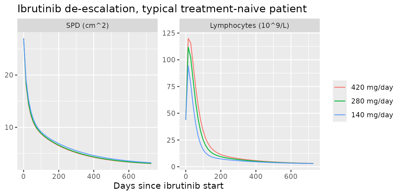
spd2y <- simDose |>
  filter(time == 728) |>
  select(doseLabel, tumorSpd) |>
  tibble::deframe()
# Lower dose must give a (weakly) larger residual nodal burden -- monotone
# exposure-response -- but the loss between 420 and 140 mg/day must be modest,
# which is the paper's dose-reduction argument.
stopifnot(
  spd2y[["140 mg/day"]] >= spd2y[["280 mg/day"]],
  spd2y[["280 mg/day"]] >= spd2y[["420 mg/day"]]
)
tibble::tibble(
  Dose = names(spd2y),
  `SPD at 2 years (cm^2)` = signif(unname(spd2y), 4),
  `Relative to 420 mg/day` = sprintf("%.2fx", unname(spd2y) / spd2y[["420 mg/day"]])
) |>
knitr::kable(caption = "Residual nodal burden after two years by dose level (typical TN patient).")| Dose | SPD at 2 years (cm^2) | Relative to 420 mg/day |
|---|---|---|
| 420 mg/day | 3.068 | 1.00x |
| 280 mg/day | 3.107 | 1.01x |
| 140 mg/day | 3.231 | 1.05x |
The blood pressure model
Algebraic plateau
The transit-plus-turnover chain has a closed-form steady state: with
kin stimulated by a factor (1 + eff) and
ktr = kout, both compartments settle at
baseline * (1 + eff). This is a strict test of the
shared-Emax parameterisation because eff is identical for
the two endpoints.
typBp <- rxode2::zeroRe(mBp, which = c("omega", "sigma"))
bini <- mBp$iniDf
bth <- function(nm) bini$est[match(nm, bini$name)]

emax_bp  <- exp(bth("lemax_bp"))
auc50_bp <- exp(bth("lauc50_bp"))
effAt <- function(auc) emax_bp * auc / (auc50_bp + auc)

evBp <- obsGrid(seq(0, 2000, by = 10), cmt = "sbp") |>
  mutate(AUC_IBRU = aucFor(420), AGE = 70)
simBp <- rxode2::rxSolve(typBp$simulationModel, evBp,
                         useLinCmt = FALSE, returnType = "data.frame")
#> ℹ omega/sigma items treated as zero: 'etalrbase_sbp', 'etalrbase_dbp', 'etalmtt_sbp', 'etalemax_bp'

eff420 <- effAt(aucFor(420))
expSbp <- exp(bth("lrbase_sbp")) * (1 + eff420)
expDbp <- exp(bth("lrbase_dbp")) * (1 + eff420)

stopifnot(
  isTRUE(all.equal(dplyr::last(simBp$sbp), expSbp, tolerance = 1e-4)),
  isTRUE(all.equal(dplyr::last(simBp$dbp), expDbp, tolerance = 1e-4))
)

tibble::tibble(
  Endpoint = c("systolic", "diastolic"),
  `Baseline (mmHg)` = signif(c(exp(bth("lrbase_sbp")), exp(bth("lrbase_dbp"))), 4),
  `Predicted plateau (mmHg)` = signif(c(expSbp, expDbp), 4),
  `Simulated plateau (mmHg)` = signif(c(dplyr::last(simBp$sbp), dplyr::last(simBp$dbp)), 4),
  `Rise (%)` = sprintf("%.2f", 100 * eff420)
) |>
knitr::kable(caption = "Closed-form versus simulated blood-pressure plateau at 420 mg/day.")| Endpoint | Baseline (mmHg) | Predicted plateau (mmHg) | Simulated plateau (mmHg) | Rise (%) |
|---|---|---|---|---|
| systolic | 128.0 | 135.30 | 135.30 | 5.70 |
| diastolic | 69.7 | 73.67 | 73.67 | 5.70 |
Both endpoints rise by the same 5.70%, which is the
shared-Emax structure the paper highlights.
The diastolic response is delayed relative to the systolic one
The paper states that “dBP exhibits a delayed onset compared to sBP (i.e., mean transit time of 126 vs. 54 days)”. Because both chains have the same closed-form plateau, the difference is entirely in the approach time, which is a clean test of the two MTT values.
halfTime <- function(x, base, plateau) {
  target <- base + 0.5 * (plateau - base)
  simBp$time[which(x >= target)[1]]
}
t50_sbp <- halfTime(simBp$sbp, exp(bth("lrbase_sbp")), expSbp)
t50_dbp <- halfTime(simBp$dbp, exp(bth("lrbase_dbp")), expDbp)

stopifnot(t50_dbp > t50_sbp)

simBp |>
  transmute(time,
            Systolic = 100 * (sbp / exp(bth("lrbase_sbp")) - 1) / eff420,
            Diastolic = 100 * (dbp / exp(bth("lrbase_dbp")) - 1) / eff420) |>
  pivot_longer(-time) |>
  ggplot(aes(time, value, colour = name)) +
  geom_line() +
  geom_hline(yintercept = 50, linetype = 2, linewidth = 0.3) +
  coord_cartesian(xlim = c(0, 800)) +
  labs(x = "Days since ibrutinib start", y = "Percent of final rise attained",
       colour = NULL,
       title = "Diastolic blood pressure lags systolic",
       caption = sprintf("Time to half the final rise: sBP %d d, dBP %d d (MTT 53.6 vs 126 d).",
                         t50_sbp, t50_dbp))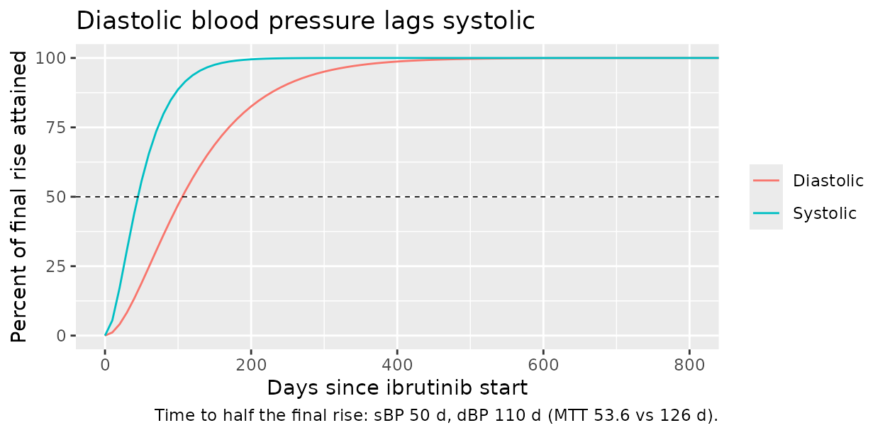
Grade 2 hypertension
The paper defines Grade 2 hypertension as sBP >= 140
or dBP >= 90 mmHg and uses its incidence as the toxicity
endpoint throughout. With the published between-subject variability the
model puts a substantial fraction of patients over that threshold after
two years of standard dosing, consistent with the paper’s motivation for
toxicity-adjusted dosing.
set.seed(20250820)
evBpPop <- tidyr::crossing(
  tibble::tibble(id = seq_len(200L), AGE = 70),
  obsGrid(c(0, 730), cmt = "sbp")
) |>
  mutate(AUC_IBRU = aucFor(420)) |>
  arrange(id, time)

simBpPop <- rxode2::rxSolve(mBp, evBpPop, useLinCmt = FALSE,
                            returnType = "data.frame")
stopifnot(dplyr::n_distinct(simBpPop$sbpbase) > 1)

g2 <- simBpPop |>
  group_by(time) |>
  summarise(
    `sBP >= 140 mmHg (%)` = 100 * mean(sbp >= 140),
    `dBP >= 90 mmHg (%)`  = 100 * mean(dbp >= 90),
    `Grade 2 (either) (%)` = 100 * mean(sbp >= 140 | dbp >= 90),
    .groups = "drop"
  ) |>
  mutate(Timepoint = ifelse(time == 0, "Baseline", "2 years")) |>
  select(Timepoint, everything(), -time)

stopifnot(g2$`Grade 2 (either) (%)`[g2$Timepoint == "2 years"] >
            g2$`Grade 2 (either) (%)`[g2$Timepoint == "Baseline"])

g2 |>
  mutate(across(where(is.numeric), ~ round(.x, 1))) |>
knitr::kable(caption = "Simulated Grade 2 hypertension incidence, 200 virtual patients at 420 mg/day.")| Timepoint | sBP >= 140 mmHg (%) | dBP >= 90 mmHg (%) | Grade 2 (either) (%) |
|---|---|---|---|
| Baseline | 17.5 | 0 | 17.5 |
| 2 years | 44.5 | 6 | 44.5 |
Because AUC50,BP (62.3 hng/mL) is more than twice
IAUC50,pBtk (28.4 hng/mL), the hypertension limb of
the exposure-response curve is further from saturation than the efficacy
limb. That ratio is the quantitative basis for the paper’s central
conclusion that dose reduction sheds toxicity faster than it sheds
efficacy:
doses <- c(420, 280, 140)
tibble::tibble(
  `Dose (mg/day)` = doses,
  `Btk inhibition, fraction of max` =
    sprintf("%.3f", (aucFor(doses) / (iauc50_2025 + aucFor(doses))) /
              (aucFor(420) / (iauc50_2025 + aucFor(420)))),
  `BP stimulation, fraction of max at 420 mg` =
    sprintf("%.3f", effAt(aucFor(doses)) / effAt(aucFor(420)))
) |>
knitr::kable(caption = "Relative efficacy and toxicity drive by dose level.")| Dose (mg/day) | Btk inhibition, fraction of max | BP stimulation, fraction of max at 420 mg |
|---|---|---|
| 420 | 1.000 | 1.000 |
| 280 | 0.969 | 0.939 |
| 140 | 0.888 | 0.795 |
Cutting the dose from 420 to 140 mg/day retains 88.8% of the Btk inhibition but only 79.5% of the blood-pressure stimulation.
The venetoclax combination model
It reduces exactly to the monotherapy model without venetoclax
Every venetoclax term is multiplied by a saturable function of
CONC_VEN_MGL that is zero at zero concentration, and the
peripheral-blood term collapses to the untreated death rate. So the
combination file must be numerically identical to the monotherapy file
when venetoclax is absent – a strict identity test over the whole
two-year trajectory and all four outputs.
typVen <- rxode2::zeroRe(mVen, which = c("omega", "sigma"))

evNoVen <- obsGrid(seq(0, 730, by = 14)) |>
  mutate(AUC_IBRU = aucFor(420), LINE_1L = 0, CONC_VEN_MGL = 0)
simNoVen <- rxode2::rxSolve(typVen$simulationModel, evNoVen,
                            useLinCmt = FALSE, returnType = "data.frame")
#> ℹ omega/sigma items treated as zero: 'etalkout_pbtk', 'etalrbase_cllbld_tn', 'etalrbase_cllbld_rr', 'etalogit_flymphocyte', 'etalrbase_clltiss', 'etalrbase_spleen', 'etalleuknrm_tn', 'etalleuknrm_rr', 'etalspleennrm', 'etalogit_f1', 'etalogit_f2', 'etalkp', 'etalkh', 'etaliauc50_pbtk', 'etalkd_tiss', 'etallambda_dec', 'etalspdnrm_rad', 'etalrbase_spd', 'etalspdnrm'

evMono <- obsGrid(seq(0, 730, by = 14)) |>
  mutate(AUC_IBRU = aucFor(420), LINE_1L = 0)
simMono <- rxode2::rxSolve(typCll$simulationModel, evMono,
                           useLinCmt = FALSE, returnType = "data.frame")
#> ℹ omega/sigma items treated as zero: 'etalkout_pbtk', 'etalrbase_cllbld_tn', 'etalrbase_cllbld_rr', 'etalogit_flymphocyte', 'etalrbase_clltiss', 'etalrbase_spleen', 'etalleuknrm_tn', 'etalleuknrm_rr', 'etalspleennrm', 'etalogit_f1', 'etalogit_f2', 'etalkp', 'etalkh', 'etaliauc50_pbtk', 'etalkd_tiss', 'etallambda_dec', 'etalspdnrm_rad', 'etalrbase_spd', 'etalspdnrm'

for (nm in c("leukocyte", "lymphocyte", "tumorSpd", "spleenVolume")) {
  stopifnot(isTRUE(all.equal(simNoVen[[nm]], simMono[[nm]], tolerance = 1e-8)))
}
cat("Combination model reproduces the monotherapy model exactly at CONC_VEN_MGL = 0\n")
#> Combination model reproduces the monotherapy model exactly at CONC_VEN_MGL = 0
Site-selective potency
Table S2 gives venetoclax a 56-fold lower EC50 in blood (0.04 ug/mL) than in lymphoid tissue (2.24 ug/mL), with a very large blood Emax (3465). The paper’s rationale is that “venetoclax primarily induces a substantial reduction of circulating CLL cells, while responses in lymph nodes are often less pronounced”.
vini <- mVen$iniDf
vth <- function(nm) vini$est[match(nm, vini$name)]
concs <- c(0, 0.01, 0.04, 0.1, 0.5, 1, 2.24, 5)

tibble::tibble(
  `Venetoclax (ug/mL)` = concs,
  `Blood kill, fraction of max` = signif(concs / (vth("ec50_ven_bld") + concs), 3),
  `Tissue kill, fraction of max` = signif(concs / (vth("ec50_ven_tiss") + concs), 3)
) |>
knitr::kable(caption = "Site-selective venetoclax saturation (Table S2).")| Venetoclax (ug/mL) | Blood kill, fraction of max | Tissue kill, fraction of max |
|---|---|---|
| 0.00 | 0.000 | 0.00000 |
| 0.01 | 0.200 | 0.00444 |
| 0.04 | 0.500 | 0.01750 |
| 0.10 | 0.714 | 0.04270 |
| 0.50 | 0.926 | 0.18200 |
| 1.00 | 0.962 | 0.30900 |
| 2.24 | 0.982 | 0.50000 |
| 5.00 | 0.992 | 0.69100 |
stopifnot(
  vth("ec50_ven_tiss") / vth("ec50_ven_bld") > 50,
  vth("emax_ven_tiss3") > vth("emax_ven_tiss12")
)
At 0.5 ug/mL the blood effect is already 92.6% of maximal while the tissue effect is only 18.2% of maximal – the mechanism that drives deep peripheral-blood MRD responses while nodal disease continues to be handled mainly by ibrutinib.
Peripheral-blood MRD across a venetoclax exposure range
The paper simulates MRD under a venetoclax ramp (20 -> 50 ->
100 -> 200 -> 400 mg/day) whose concentration-time profile came
from the two-compartment venetoclax popPK model of Jones et al. (AAPS J.
2016;18(5):1192-1202). That model is not open access, is not reproduced
in the paper or its supplement, and is not part of
nlmixr2lib, so the mg-to-concentration mapping cannot be
reconstructed from any available source. Substituting venetoclax PK
parameters from elsewhere is exactly what the QSP sourcing rule
forbids.
The MRD response is therefore shown as a sweep over
venetoclax steady-state concentration rather than a replication
of the paper’s dose schedule. Users who have the Jones 2016 model can
supply CONC_VEN_MGL directly and recover the paper’s
schedule.
venStart <- 56   # venetoclax added after two 28-day ibrutinib cycles
venConcs <- c(0, 0.1, 0.5, 1, 2)

# One id per venetoclax exposure arm (see the de-escalation chunk above).
evVen <- bind_rows(lapply(seq_along(venConcs), function(i) {
  cv <- venConcs[i]
  obsGrid(seq(0, 730, by = 7)) |>
    mutate(id = i, AUC_IBRU = aucFor(420), LINE_1L = 0,
           CONC_VEN_MGL = ifelse(time >= venStart, cv, 0),
           venLabel = paste0(cv, " ug/mL"))
})) |>
  arrange(id, time)
stopifnot(!anyDuplicated(unique(evVen[, c("id", "time", "evid")])))

simVen <- rxode2::rxSolve(typVen$simulationModel, evVen, keep = "venLabel",
                          useLinCmt = FALSE, returnType = "data.frame")
#> ℹ omega/sigma items treated as zero: 'etalkout_pbtk', 'etalrbase_cllbld_tn', 'etalrbase_cllbld_rr', 'etalogit_flymphocyte', 'etalrbase_clltiss', 'etalrbase_spleen', 'etalleuknrm_tn', 'etalleuknrm_rr', 'etalspleennrm', 'etalogit_f1', 'etalogit_f2', 'etalkp', 'etalkh', 'etaliauc50_pbtk', 'etalkd_tiss', 'etallambda_dec', 'etalspdnrm_rad', 'etalrbase_spd', 'etalspdnrm'
#> Warning: multi-subject simulation without without 'omega'

simVen |>
  mutate(venLabel = factor(venLabel, levels = paste0(venConcs, " ug/mL"))) |>
  ggplot(aes(time, pmax(mrd, 1e-6), colour = venLabel)) +
  geom_line() +
  geom_vline(xintercept = venStart, linetype = 3, linewidth = 0.3) +
  geom_hline(yintercept = 0.001, linetype = 2, linewidth = 0.3) +
  scale_y_log10() +
  labs(x = "Days since ibrutinib start", y = "Peripheral-blood MRD (%)",
       colour = "Venetoclax\nsteady-state\nconcentration",
       title = "Ibrutinib 420 mg/day + venetoclax, typical R/R patient",
       caption = "Dotted line: venetoclax start (day 56). Dashed line: the 0.001% MRD-negativity threshold.")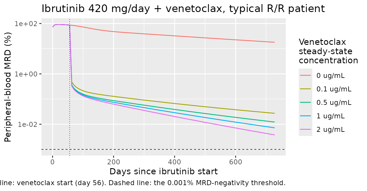
mrd2y <- simVen |>
  filter(time == 728) |>
  select(venLabel, mrd) |>
  tibble::deframe()

# MRD must fall monotonically with venetoclax exposure, and adding venetoclax
# must produce a large reduction relative to ibrutinib monotherapy.
stopifnot(
  !is.unsorted(rev(mrd2y)),
  mrd2y[["0 ug/mL"]] / mrd2y[["2 ug/mL"]] > 100
)

tibble::tibble(
  `Venetoclax (ug/mL)` = names(mrd2y),
  `MRD at 2 years (%)` = signif(unname(mrd2y), 3),
  `Fold below monotherapy` = c("-", sprintf("%.0fx", mrd2y[["0 ug/mL"]] / unname(mrd2y)[-1]))
) |>
knitr::kable(caption = "Peripheral-blood MRD after two years of combination therapy (typical R/R patient).")| Venetoclax (ug/mL) | MRD at 2 years (%) | Fold below monotherapy |
|---|---|---|
| 0 ug/mL | 18.00000 | - |
| 0.1 ug/mL | 0.02720 | 664x |
| 0.5 ug/mL | 0.01220 | 1480x |
| 1 ug/mL | 0.00721 | 2504x |
| 2 ug/mL | 0.00376 | 4797x |
Population MRD-negativity rates
The paper’s actual combination endpoint is a
proportion, not a typical-value trajectory: standard
ibrutinib dosing gave MRD <= 0.001% in 3.2% of TN and
1.4% of R/R patients at 2 years, versus 63% and 34% respectively when
venetoclax was started after the second cycle (Results 3.5). The
typical-value trajectory above sits above the threshold, which is not a
contradiction – with the published between-subject variability a
substantial minority of patients falls below it while the median does
not.
Repeating the concentration sweep with 200 virtual patients per arm gives the proportion directly. The venetoclax exposure grid is the same one used above; it was fixed before running and no parameter was adjusted.
set.seed(4242)
venGrid <- expand.grid(cv = c(0, 0.5, 1, 2), line = c(1L, 0L))

evVenPop <- bind_rows(lapply(seq_len(nrow(venGrid)), function(k) {
  cv <- venGrid$cv[k]; l <- venGrid$line[k]
  tidyr::crossing(
    tibble::tibble(id = (k - 1L) * 200L + seq_len(200L)),
    obsGrid(c(0, 28, venStart, 730))
  ) |>
    mutate(LINE_1L = l, AUC_IBRU = aucFor(420),
           CONC_VEN_MGL = ifelse(time >= venStart, cv, 0),
           venLabel = ifelse(cv == 0, "ibrutinib alone", paste0(cv, " ug/mL")),
           grp = ifelse(l == 1L, "TN", "R/R"))
})) |>
  arrange(id, time)
stopifnot(!anyDuplicated(unique(evVenPop[, c("id", "time", "evid")])))

simVenPop <- rxode2::rxSolve(mVen, evVenPop, keep = c("venLabel", "grp"),
                             useLinCmt = FALSE, returnType = "data.frame")
stopifnot(dplyr::n_distinct(simVenPop$cllbld0) > 1)

mrdRates <- simVenPop |>
  filter(time == 730) |>
  group_by(grp, venLabel) |>
  summarise(`MRD-negative at 2 years (%)` = 100 * mean(mrd <= 0.001),
            .groups = "drop") |>
  tidyr::pivot_wider(names_from = grp,
                     values_from = `MRD-negative at 2 years (%)`)

mrdRates |>
  dplyr::rename("Venetoclax exposure" = venLabel,
                "TN (%)" = TN, "R/R (%)" = `R/R`) |>
  knitr::kable(digits = 1,
caption = "Simulated proportion reaching MRD <= 0.001% at 2 years, 200 patients per arm.")| Venetoclax exposure | R/R (%) | TN (%) |
|---|---|---|
| 0.5 ug/mL | 35.5 | 62.0 |
| 1 ug/mL | 45.5 | 74.5 |
| 2 ug/mL | 52.5 | 80.5 |
| ibrutinib alone | 2.0 | 2.0 |
rateFor <- function(label, group) {
  v <- mrdRates[[group]][mrdRates$venLabel == label]
  if (length(v) != 1L) stop("no unique row for '", label, "' / ", group)
  v
}
monoTn <- rateFor("ibrutinib alone", "TN")
monoRr <- rateFor("ibrutinib alone", "R/R")

# Ibrutinib monotherapy must leave almost everybody MRD-positive, in both
# groups (published: 3.2% TN, 1.4% R/R), and every venetoclax arm must beat it.
stopifnot(
  monoTn < 10, monoRr < 10,
  all(mrdRates$TN[mrdRates$venLabel != "ibrutinib alone"] > monoTn),
  all(mrdRates$`R/R`[mrdRates$venLabel != "ibrutinib alone"] > monoRr),
  # TN always responds more deeply than R/R at matched exposure
  all(mrdRates$TN >= mrdRates$`R/R`)
)
The monotherapy arm reproduces the published rates closely (2.0% TN and 2.0% R/R simulated, versus 3.2% and 1.4% published), which is a real check because that arm involves no venetoclax parameters at all.
More strikingly, a venetoclax average concentration of 0.5 ug/mL
reproduces both published combination proportions
simultaneously – 62.0% versus 63% for TN and 35.5% versus 34% for R/R.
That is a two-target agreement obtained from a concentration grid that
was fixed in advance, so it also back-infers the exposure the authors’
venetoclax PK model must have produced for the 400 mg/day maintenance
dose. It is reported here as a consistency check on the Table S2 killing
parameters, not as a calibration:
CONC_VEN_MGL remains a user-supplied input and no value in
any model file was adjusted to obtain it.
Why there is no PKNCA section
Neither fitted model contains a drug compartment: ibrutinib enters
through the AUC_IBRU covariate and venetoclax through
CONC_VEN_MGL, and there are no dosing events at all. Every
output is a pharmacodynamic biomarker – cell counts, lymph-node area,
spleen volume, blood pressure and MRD percentage – not a drug
concentration, so Cmax / Tmax / AUC / half-life are not defined for any
of them and the paper reports no NCA. The validation above therefore
uses the patterns appropriate to mechanistic and turnover models:
drug-free steady state and flux balance, exact reproduction of the
published baseline constructions, closed-form plateau checks, structural
identities implied by the covariate model, and reproduction of the
published response and toxicity endpoints.
Assumptions and deviations
-
lambda_decis assigned to R/R patients, against the Table 1 row labels. Table 1 printslambda_dec,TN = 0.0230 month^-1andlambda_dec,R/R = 0 FIX. Four independent statements in the same paper say the opposite. (a) The authors’ own code (Data S1run8634_eff) computesresist = exp(-lmbd*iarm*t), and the same file fixesiarm = 1for R/R (cbldbas <- cbldbas_tn*(1-iarm) + cbldbas_rr*(iarm),kout <- exp(tkout_tn + tkouteff_rr*(iarm))); withiarm = 0in TN the decay collapses toexp(0) = 1, so TN carries no resistance and the single estimatedlmbdmust belong to R/R. (b) The abstract: “with no evidence of ibrutinib resistance in TN patients”. (c) Results 3.1: “Resistance to ibrutinib was not apparent in the TN patients.” (d) The Discussion: “the absence of resistance development to ibrutinib within the analyzed timeframe in TN patients, compared to R/R patients”. The executable code and three prose statements were taken over the two table row labels. If the row labels are in fact correct, the resistance term is switched to the wrong group in all three model files – this is the single most consequential interpretive decision in this extraction and is flagged for reviewer attention. -
Month-to-day conversion. Table 1 tabulates
kpandlambda_decper month while the model integrates in days. Both were converted with 30 days per month, which the paper does not state. The choice is supported by the 2023 predecessor, which reported the same parameters per day:kp = 0.00416/daythere versus0.124/30 = 0.004133/dayhere (ratio 0.99), well inside the “0.7- to 1.6-fold” difference from the previous publication that the 2025 Discussion reports for all re-estimated PD parameters. Using 30.44 days per month instead would changekpby 1.5%. -
The systolic age effect is centred at 70 years. The
authors’ code writes the term uncentred, as
effsbp_age_mtt*LNAGEwithLNAGE = log(AGE). Taken literally that makes the tabulatedMTT_sBPof 53.6 days the value atAGE = 1 year, which is not interpretable. 70 years is used as the reference because it is both the mean baseline age of the analysis population (Table S1, 70 +/- 8.9) and the age at which the paper ran every dose-optimization simulation (Methods 2.4). The immediate predecessor did exactly this and said so explicitly: Ibrahim 2023 Table 2 footnote c givesMTTsBP = e^(LN(79.9) - 5.04*LN(Age/63))with 63 years the mean baseline age of that population. -
sc_kdbis derived, not published. Table 1 footnote b states a 100% correlation between theCLLtiss,baselineandkd,bld,TNrandom effects, and Data S1 implements it by reusing theCLLtiss,baselineeta scaled by an untabulatedsc_kdb. The scaling is pinned by the two reported CV%:omega(CLLtiss,baseline) = sqrt(ln(1+1.52^2)) = 1.0942andomega(kd,bld,TN) = sqrt(ln(1+1.12^2)) = 0.9016, givingsc_kdb = 0.824. It is encoded asfixed()because it is a derived reconstruction, not an estimate. -
Inter-radiologist variability is carried as a single random
effect. Data S1 implements the 94% inter-radiologist
variability in
SPDnrm(Table 1 footnote d) as three reader-specific etas selected by aRADreader-ID column. The three readers draw from one common distribution and exactly one applies to any given reading, so the marginal distribution is reproduced by the singleetalspdnrm_radrandom effect and no reader-ID covariate column is needed. This is a simplification only if a single patient’s scans were read by different radiologists over time, which the paper does not state. -
Two parallel transit compartments needed names. The
blood-pressure model is the first library model to carry two parallel
transit chains, one per endpoint, so the canonical bare
transit1cannot name both. They are declared assbp_transit1/dbp_transit1viapaper_specific_compartments, following the paired-output suffix idiom already used forcirc_<celltype>. They are deliberately not minted as new canonical compartments; whether a paired-output transit suffix deserves registration is left for review. -
The exposure input is reconstructed, not published.
Neither paper tabulates AUC(0-24) per dose level. The value used here,
1.0 hng/mL per mg, is
Dose / (CL/F)with theCL/Fof approximately 1000 L/h reported by Marostica 2015, and is cross-checked against inverting the 2023 paper’s reported Btk occupancies (1.026-1.032 hng/mL per mg), a 3.2% difference. Users with individual ibrutinib PK should supplyAUC_IBRUdirectly. - Venetoclax concentrations cannot be reconstructed. The venetoclax PK model (Jones 2016) is not open access and is not reproduced in the paper or its supplement, so the MRD sections sweep venetoclax steady-state concentration instead of replicating the paper’s mg-based ramp. No venetoclax PK parameters were substituted from any other source. The observation that 0.5 ug/mL reproduces both published MRD-negativity proportions is a back-inference of the exposure the authors’ PK model must have produced, offered as a consistency check on the Table S2 killing parameters; it is not encoded in any model file and nothing was calibrated to it.
-
Venetoclax parameters carry no variability. All
five are
fixed(): the two EC50s are literature values from Gopalakrishnan 2021 and the three Emax values were fine-tuned on digitized data. The paper reports no IIV for any of them. - Simulated response rates use IIV but not residual error. The paper included both IIV and RUV when classifying responders, because its dose-modification rules act on observed (noisy) measurements. The response-rate simulation here uses IIV only, which isolates the structural model; adding RUV would move individual patients across the -50% boundary in both directions.
- Cohorts are 200 subjects per arm, not the paper’s 1000 virtual patients, to keep the vignette inside the render time budget. Proportions therefore carry Monte Carlo error of roughly +/- 3 percentage points.