Linezolid (Xu 2024) • nlmixr2lib

Model and source

Citation: Xu J, Chen X, Zhang Q, Zhuang Z, Yuan Y, Duan L, Shi L, Zhu C, Li J, Lu J, Yu Y, Tang L. (2024). Population Pharmacokinetic/Pharmacodynamic Study of Linezolid in Hospital-Acquired Pneumonia Patients with Renal Insufficiency. Drug Design, Development and Therapy 18:5073-5086. doi:10.2147/DDDT.S474470
Description: Population PK model for intravenous linezolid in hospital-acquired pneumonia patients with renal insufficiency (Xu 2024). One-compartment disposition with linear elimination; clearance carries power-model effects of age (exponent -0.56, reference 82 years) and Cockcroft-Gault creatinine clearance (exponent 0.50, reference 42 mL/min). Volume of distribution is a typical value with no inter-individual variability; inter-individual variability was estimated on clearance only, and residual variability is additive.
Article: https://doi.org/10.2147/DDDT.S474470

Xu 2024 is a two-part retrospective study at a single Chinese centre. The first part is a comparative pharmacodynamic analysis (clinical and microbiological efficacy, safety, and trough-target attainment) of linezolid versus teicoplanin; it is a statistical comparison of clinical outcomes and contains no pharmacodynamic model, so nothing from it is packaged here. The second part is the population PK analysis that this vignette validates: a one-compartment model with linear elimination fit to 207 linezolid serum concentrations from 166 patients with hospital-acquired pneumonia and renal insufficiency.

Population

The PK analysis used 207 linezolid serum concentrations from 166 adults with hospital-acquired pneumonia (2016 ATS/IDSA criteria) and renal insufficiency, defined per the 2010 FDA guidance as a Cockcroft-Gault creatinine clearance below 90 mL/min. Patients on renal replacement therapy, with a baseline platelet count below 75000/uL, with severe hepatic impairment, or with known bleeding disorders were excluded. Linezolid was given as 600 mg every 12 h by intravenous infusion per the package label, with clinicians free to adjust the regimen on the basis of steady-state troughs. Samples were predominantly steady-state troughs drawn 30 min or immediately before the next dose and at least 48 h after therapy started; the authors note (Discussion, limitation four) that this limits resolution of the distribution phase. Concentrations were measured by HPLC-MS/MS over a 0.5-50.0 mg/L linear range.

The PPK cohort’s own baseline characteristics are in supplementary Table S1 (n = 166): 73.5% male; age median (IQR) 82.0 (75.0, 89.0) years; weight 60.0 (55.0, 65.0) kg; serum creatinine 106.2 (70.2, 181.7) umol/L; CrCL 42.0 (29.2, 54.0) mL/min; albumin 31.8 (28.2, 34.5) g/L; treatment duration 9.0 (8.0, 12.0) days; respiratory failure 47.6%, septic shock 29.5%, MODS 14.5%. Table S1 also tabulates the companion pharmacodynamic study’s linezolid arm (n = 81) side by side and finds no significant difference on any characteristic (all P >= 0.105).

The two centering values printed in the final CL equation are exactly the PPK cohort’s own medians – 82 years against a Table S1 median age of 82.0 years, and 42.0 mL/min against a Table S1 median CrCL of 42.0 mL/min. Since Table S1 and the equation are separate objects in separate files, that coincidence is an independent check that the equation has been transcribed correctly here.

In the main text, MRSA was the most frequent respiratory isolate (69/87 samples, 79.3%) and 27.6% of patients had a mixed Gram-positive/Gram-negative respiratory infection.

The same information is available programmatically via the model’s population metadata (readModelDb("Xu_2024_linezolid")()$population).

Source trace

The per-parameter origin is recorded as an in-file comment next to each ini() entry in inst/modeldb/specificDrugs/Xu_2024_linezolid.R. The table below collects them in one place for review. All page numbers refer to Drug Des Devel Ther 2024;18:5073-5086.

Equation / parameter	Value	Source location
Structural model: one compartment, linear elimination	n/a	Results, “PPK Study” (p. 5077): “Linezolid pharmacokinetics was adequately described by one compartment disposition model with linear elimination.”
Intravenous infusion into `central`, 1 h	n/a	Methods, “Dosing Regimen” (p. 5075) and “PPK Study” (p. 5076): “The infusion time was set to 1 h.”
`lcl` = log(2.7)	CL = 2.7 L/h	Table 3 (p. 5078), TVCL; final-model equation p. 5078
`lvc` = log(57.1)	V = 57.1 L	Table 3 (p. 5078), TVv; final-model equation p. 5078
`e_age_cl`	-0.56	Final-model equation p. 5078, `(age/82)^-0.56`. Table 3 reports theta_Age = -0.6, i.e. the same value rounded to one decimal place.
`e_crcl_cl`	0.50	Final-model equation p. 5078, `(CrCL/42.0)^0.50`. Table 3 reports theta_CrCL = 0.5.
Age centering value	82 years	Final-model equation p. 5078; equals the PPK-cohort median age of 82.0 (75.0, 89.0) y in supplementary Table S1
CrCL centering value	42.0 mL/min	Final-model equation p. 5078; equals the PPK-cohort median CrCL of 42.0 (29.2, 54.0) mL/min in supplementary Table S1
PPK-cohort demographics	n = 166	Supplementary Table S1
Covariate model-building path	CL-CrCL, CL-age only	Supplementary Table S2 (basic model OFV 1327.8; full covariate model 1266.5; backward elimination +6.9 removing CL-age, +50.7 removing CL-CrCL)
`etalcl` (variance)	0.1	Table 3 (p. 5078), `omega^2 CL`; table footnote defines it as “variance of inter-individual variability of clearance”. Eta shrinkage 23.3%.
No IIV on V	n/a	Final-model equation p. 5078 carries `exp(eta_CL)` on CL only; `V (L) = 57.1` has no random-effect term, and Table 3 reports no `omega^2 V`.
`addSd`	3.4 mg/L	Table 3 (p. 5078), `sigma`; table footnote defines sigma as “square root of residual variability”. Results, “PPK Study”: “The additive error model was found to best fit the data.”
`AGE` covariate on CL	power model	Final-model equation p. 5078
`CRCL` covariate on CL	power model	Final-model equation p. 5078; Cockcroft-Gault per Methods, “Study Design and Patients” (p. 5074)
`WT` screened, not retained	n/a	Discussion (p. 5082): “Body weight was not identified as a significant covariate affecting linezolid clearance in our study”
Published PTA reference values	Table 4	Table 4 (p. 5080), “Simulated Probability of Attaining Linezolid Cmin Stratified by Renal Function and Age”
Cmin target range	2-8 mg/L	Methods, “PPK Study” (p. 5076) and “Comparative Pharmacodynamic Study” (p. 5075)

Virtual cohort

Original observed data are not publicly available. The cohort below reproduces the covariate grid of the paper’s own Monte Carlo analysis (Table 4): a renal sweep at the cohort-median age (CrCL 90, 60, 45, 30 and 15 mL/min at age 80 y) and an age sweep at the cohort-median renal function (age 100, 90, 70, 50 and 30 y at CrCL 40 mL/min), each crossed with the four simulated regimens (600, 400, 300 and 200 mg every 12 h as 1 h infusions).

That is 40 arms. The paper simulated 1000 virtual individuals; this vignette uses 200 per arm, which is the per-arm cap for nlmixr2lib validation vignettes and gives a Monte Carlo standard error of roughly 3.5 percentage points on each attainment probability.

set.seed(20241108)

n_per_arm <- 200L
tau <- 12 # dosing interval (h)
t_inf <- 1 # infusion duration (h), Xu 2024 Methods

# The 10 covariate scenarios of Xu 2024 Table 4: rows flagged "a" use the
# approximate median age (80 y) and sweep CrCL; rows flagged "b" use the
# approximate median CrCL (40 mL/min) and sweep age.
scenarios <- dplyr::bind_rows(
  tibble::tibble(sweep = "Renal function (age 80 y)", AGE = 80, CRCL = c(90, 60, 45, 30, 15)),
  tibble::tibble(sweep = "Age (CrCL 40 mL/min)", AGE = c(100, 90, 70, 50, 30), CRCL = 40)
)

doses <- c(600, 400, 300, 200)

arms <- tidyr::crossing(scenarios, dose_mg = doses) |>
  dplyr::mutate(
    arm = sprintf("%d mg q12h | age %g y | CrCL %g mL/min", dose_mg, AGE, CRCL),
    id_offset = (dplyr::row_number() - 1L) * n_per_arm
  )

# Helper: one arm's event table. Steady state is requested directly with
# ss = 1 / ii = tau rather than by dosing forward for many half-lives; the
# terminal half-life reaches ~50 h in the low-CrCL / low-eta corner of this
# cohort, so an explicit multiple-dose run-in would have to be very long.
make_arm <- function(dose_mg, AGE, CRCL, arm, id_offset, sweep) {
  ids <- id_offset + seq_len(n_per_arm)
  subj <- tibble::tibble(
    id = ids, AGE = AGE, CRCL = CRCL, dose_mg = dose_mg, arm = arm, sweep = sweep
  )
  dose_rows <- subj |>
    dplyr::mutate(
      time = 0, evid = 1L, cmt = "central",
      amt = dose_mg, rate = dose_mg / t_inf,
      ii = tau, ss = 1L
    )
  obs_rows <- subj |>
    tidyr::crossing(time = seq(0, tau, by = 0.5)) |>
    dplyr::mutate(
      evid = 0L, cmt = "central",
      amt = NA_real_, rate = NA_real_, ii = 0, ss = 0L
    )
  dplyr::bind_rows(dose_rows, obs_rows) |>
    dplyr::arrange(id, time, dplyr::desc(evid))
}

events <- do.call(
  dplyr::bind_rows,
  Map(
    make_arm,
    arms$dose_mg, arms$AGE, arms$CRCL, arms$arm, arms$id_offset, arms$sweep
  )
)

# Cheap regression guard: cohort IDs must be disjoint across arms, otherwise
# rxSolve silently merges subjects and sums their doses.
stopifnot(!anyDuplicated(unique(events[, c("id", "time", "evid")])))
stopifnot(dplyr::n_distinct(events$id) == nrow(arms) * n_per_arm)
nrow(events)
#> [1] 208000

Simulation

mod <- readModelDb("Xu_2024_linezolid")

sim <- rxode2::rxSolve(
  mod,
  events = events,
  keep = c("arm", "sweep", "dose_mg", "AGE", "CRCL")
) |>
  as.data.frame()
#> ℹ parameter labels from comments will be replaced by 'label()'

str(sim[, c("id", "time", "central", "Cc", "cl", "arm")], max.level = 1)
#> 'data.frame':    200000 obs. of  6 variables:
#>  $ id     : int  1 1 1 1 1 1 1 1 1 1 ...
#>  $ time   : num  0 0.5 1 1.5 2 2.5 3 3.5 4 4.5 ...
#>  $ central: num  106 199 288 275 263 ...
#>  $ Cc     : num  1.85 3.48 5.04 4.82 4.6 ...
#>  $ cl     : num  5.19 5.19 5.19 5.19 5.19 ...
#>  $ arm    : chr  "200 mg q12h | age 30 y | CrCL 40 mL/min" "200 mg q12h | age 30 y | CrCL 40 mL/min" "200 mg q12h | age 30 y | CrCL 40 mL/min" "200 mg q12h | age 30 y | CrCL 40 mL/min" ...

Typical-value check against the printed clearance equation

Before any distributional comparison, confirm that the packaged model reproduces the printed equation CL = 2.7 * (age/82)^-0.56 * (CrCL/42.0)^0.50 exactly at the typical value. zeroRe() is applied to a fresh readModelDb() result so the stochastic model object above is left untouched.

mod_typical <- rxode2::zeroRe(readModelDb("Xu_2024_linezolid"))
#> ℹ parameter labels from comments will be replaced by 'label()'

sim_typical <- rxode2::rxSolve(
  mod_typical,
  events = events |> dplyr::filter(id %in% (arms$id_offset + 1L)),
  keep = c("arm", "sweep", "dose_mg", "AGE", "CRCL")
) |>
  as.data.frame()
#> ℹ omega/sigma items treated as zero: 'etalcl'
#> Warning: multi-subject simulation without without 'omega'

cl_check <- sim_typical |>
  dplyr::group_by(AGE, CRCL) |>
  dplyr::summarise(cl_model = mean(cl), vc_model = mean(vc), .groups = "drop") |>
  dplyr::mutate(
    cl_equation = 2.7 * (AGE / 82)^-0.56 * (CRCL / 42.0)^0.50,
    abs_pct_diff = 100 * abs(cl_model - cl_equation) / cl_equation
  )

stopifnot(max(cl_check$abs_pct_diff) < 1e-6)
stopifnot(all(abs(cl_check$vc_model - 57.1) < 1e-9))

cl_check |>
  dplyr::arrange(AGE, CRCL) |>
  dplyr::rename(
    "Age (y)" = AGE, "CrCL (mL/min)" = CRCL,
    "CL from model (L/h)" = cl_model, "V from model (L)" = vc_model,
    "CL from Xu 2024 equation (L/h)" = cl_equation,
    "|% diff|" = abs_pct_diff
  ) |>
  knitr::kable(
    digits = 4,
    caption = paste(
      "Typical-value clearance and volume from the packaged model versus the",
      "final-model equation printed on p. 5078 of Xu 2024. Agreement is exact",
      "to machine precision at all 10 covariate scenarios."
    )
  )

Typical-value clearance and volume from the packaged model versus the final-model equation printed on p. 5078 of Xu 2024. Agreement is exact to machine precision at all 10 covariate scenarios.
Age (y)	CrCL (mL/min)	CL from model (L/h)	V from model (L)	CL from Xu 2024 equation (L/h)
30	40	4.6272	57.1	4.6272
50	40	3.4760	57.1	3.4760
70	40	2.8791	57.1	2.8791
80	15	1.6360	57.1	1.6360
80	30	2.3137	57.1	2.3137
80	45	2.8337	57.1	2.8337
80	60	3.2721	57.1	3.2721
80	90	4.0074	57.1	4.0074
90	40	2.5011	57.1	2.5011
100	40	2.3578	57.1	2.3578

Replicate published figures

Xu 2024’s model-diagnostic figures (Figures 2 and 3, goodness-of-fit; Figure 4, prediction-corrected VPC) are all plotted against the observed concentrations, which are not public, so they cannot be reproduced directly. The panel below is the closest available analogue: the simulated steady-state concentration-time profile over one dosing interval, with the paper’s 2-8 mg/L trough target band overlaid, for the renal sweep at the cohort-median age.

sim |>
  dplyr::filter(sweep == "Renal function (age 80 y)") |>
  dplyr::group_by(time, dose_mg, CRCL) |>
  dplyr::summarise(
    Q05 = quantile(Cc, 0.05, na.rm = TRUE),
    Q50 = quantile(Cc, 0.50, na.rm = TRUE),
    Q95 = quantile(Cc, 0.95, na.rm = TRUE),
    .groups = "drop"
  ) |>
  dplyr::mutate(dose_lab = factor(paste0(dose_mg, " mg q12h"),
    levels = paste0(doses, " mg q12h")
  )) |>
  ggplot(aes(time, Q50, colour = factor(CRCL), fill = factor(CRCL))) +
  annotate("rect",
    xmin = -Inf, xmax = Inf, ymin = 2, ymax = 8,
    fill = "grey70", alpha = 0.35
  ) +
  geom_ribbon(aes(ymin = Q05, ymax = Q95), alpha = 0.15, colour = NA) +
  geom_line(linewidth = 0.7) +
  facet_wrap(~dose_lab) +
  scale_y_log10() +
  labs(
    x = "Time within the steady-state dosing interval (h)",
    y = "Linezolid concentration (mg/L)",
    colour = "CrCL (mL/min)", fill = "CrCL (mL/min)",
    title = "Steady-state profiles at age 80 y",
    caption = paste(
      "Median with 5th-95th percentile band, 200 subjects per arm.",
      "Grey band is the 2-8 mg/L trough target of Xu 2024.",
      "Analogue of Figure 4 of Xu 2024 (the published pcVPC is plotted",
      "against observed data that are not public)."
    )
  ) +
  theme_bw() +
  theme(legend.position = "bottom")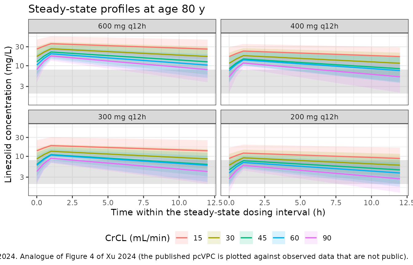

sim |>
  dplyr::filter(sweep == "Age (CrCL 40 mL/min)") |>
  dplyr::group_by(time, dose_mg, AGE) |>
  dplyr::summarise(
    Q50 = quantile(Cc, 0.50, na.rm = TRUE),
    .groups = "drop"
  ) |>
  dplyr::mutate(dose_lab = factor(paste0(dose_mg, " mg q12h"),
    levels = paste0(doses, " mg q12h")
  )) |>
  ggplot(aes(time, Q50, colour = factor(AGE))) +
  annotate("rect",
    xmin = -Inf, xmax = Inf, ymin = 2, ymax = 8,
    fill = "grey70", alpha = 0.35
  ) +
  geom_line(linewidth = 0.7) +
  facet_wrap(~dose_lab) +
  scale_y_log10() +
  labs(
    x = "Time within the steady-state dosing interval (h)",
    y = "Median linezolid concentration (mg/L)",
    colour = "Age (y)",
    title = "Steady-state median profiles at CrCL 40 mL/min",
    caption = paste(
      "The negative age exponent (-0.56) lowers clearance, and so raises",
      "exposure, with increasing age. Grey band is the 2-8 mg/L target."
    )
  ) +
  theme_bw() +
  theme(legend.position = "bottom")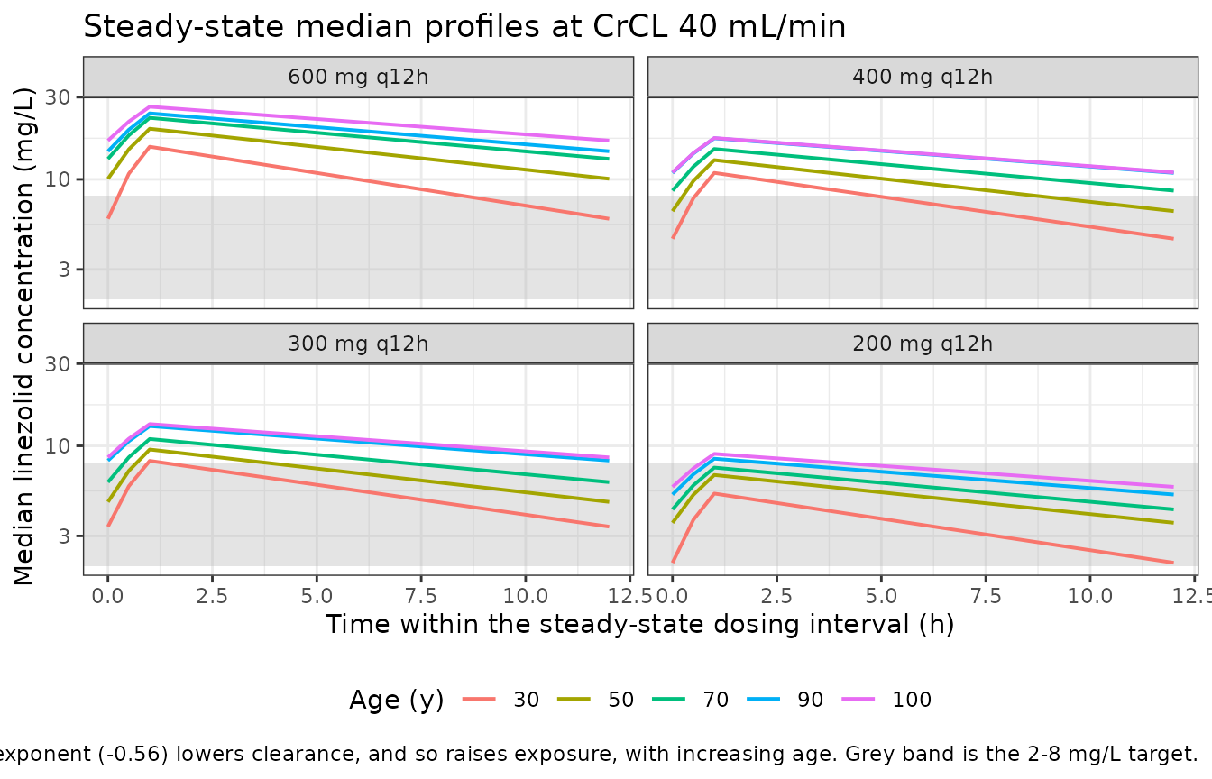

PKNCA validation

The paper’s samples were steady-state troughs, and its quantitative simulation result (Table 4) is expressed entirely in terms of the steady-state trough Cmin. PKNCA is therefore used with the steady-state recipe over the final dosing interval: it supplies ctrough (the concentration at the end of the interval, which is the paper’s Cmin definition of “30 min or immediately prior to the next dose”), cmin, cmax, cav and auclast over tau.

sim_nca <- sim |>
  dplyr::filter(!is.na(Cc)) |>
  dplyr::select(id, time, Cc, arm)

sim_nca <- sim_nca |>
  dplyr::distinct(id, arm, time, .keep_all = TRUE) |>
  dplyr::arrange(id, arm, time)

# A missing time-zero row is the most common PKNCA defect in this repo (it
# triggers "Requesting an AUC range starting (0) before the first measurement"
# once per subject). The steady-state event table observes at time 0 by
# construction, and at steady state that row is the genuine pre-dose trough --
# NOT zero -- so it must not be synthesised. Assert it is present instead.
stopifnot(
  nrow(dplyr::filter(sim_nca, time == 0)) == dplyr::n_distinct(sim_nca$id),
  all(dplyr::filter(sim_nca, time == 0)$Cc > 0)
)

conc_obj <- PKNCA::PKNCAconc(
  sim_nca, Cc ~ time | arm + id,
  concu = "mg/L", timeu = "h"
)

dose_df <- events |>
  dplyr::filter(evid == 1) |>
  dplyr::select(id, time, amt, arm)

dose_obj <- PKNCA::PKNCAdose(
  dose_df, amt ~ time | arm + id,
  doseu = "mg"
)

intervals <- data.frame(
  start = 0,
  end = tau,
  cmax = TRUE,
  tmax = TRUE,
  cmin = TRUE,
  ctrough = TRUE,
  cav = TRUE,
  auclast = TRUE
)

nca_res <- PKNCA::pk.nca(
  PKNCA::PKNCAdata(conc_obj, dose_obj, intervals = intervals)
)

nca_tbl <- as.data.frame(nca_res$result)
head(nca_tbl)
#>                                        arm   id start end PPTESTCD   PPORRES
#> 1 200 mg q12h | age 100 y | CrCL 40 mL/min 3201     0  12  auclast 86.572940
#> 2 200 mg q12h | age 100 y | CrCL 40 mL/min 3201     0  12     cmax  8.925339
#> 3 200 mg q12h | age 100 y | CrCL 40 mL/min 3201     0  12     cmin  5.719393
#> 4 200 mg q12h | age 100 y | CrCL 40 mL/min 3201     0  12     tmax  1.000000
#> 5 200 mg q12h | age 100 y | CrCL 40 mL/min 3201     0  12      cav  7.214412
#> 6 200 mg q12h | age 100 y | CrCL 40 mL/min 3201     0  12  ctrough  5.719393
#>   exclude PPORRESU
#> 1    <NA>   h*mg/L
#> 2    <NA>     mg/L
#> 3    <NA>     mg/L
#> 4    <NA>        h
#> 5    <NA>     mg/L
#> 6    <NA>     mg/L

Steady-state closed-form gate

Xu 2024 publishes no NCA table, so there is no set of published Cmax / Tmax / AUC / half-life values to compare against. The available independent check is a closed-form one: for a one-compartment model at steady state, the average concentration over a dosing interval must equal Dose / (tau * CL) exactly, regardless of volume or infusion duration. This gates the PKNCA setup, the event table, and the model’s clearance parameterisation together.

cav_sim <- nca_tbl |>
  dplyr::filter(PPTESTCD == "cav") |>
  dplyr::left_join(
    sim |> dplyr::distinct(id, arm, dose_mg, AGE, CRCL),
    by = c("id", "arm")
  ) |>
  dplyr::left_join(
    sim |> dplyr::distinct(id, cl),
    by = "id"
  ) |>
  dplyr::mutate(cav_closed_form = dose_mg / (tau * cl))

cav_gate <- cav_sim |>
  dplyr::mutate(pct_diff = 100 * (PPORRES - cav_closed_form) / cav_closed_form) |>
  dplyr::group_by(dose_mg) |>
  dplyr::summarise(
    n = dplyr::n(),
    median_pct_diff = median(pct_diff),
    max_abs_pct_diff = max(abs(pct_diff)),
    .groups = "drop"
  )

# PKNCA's cav comes from a linear-up/log-down trapezoidal AUC on a 0.5 h grid,
# so a small positive bias against the exact closed form is expected; anything
# beyond a couple of percent would indicate a real defect.
stopifnot(max(cav_gate$max_abs_pct_diff) < 2)

cav_gate |>
  dplyr::rename(
    "Dose (mg q12h)" = dose_mg,
    "n subjects" = n,
    "Median % diff vs Dose/(tau*CL)" = median_pct_diff,
    "Max |% diff|" = max_abs_pct_diff
  ) |>
  knitr::kable(
    digits = 3,
    caption = paste(
      "Closed-form gate: PKNCA's steady-state average concentration versus the",
      "exact one-compartment identity Cav,ss = Dose / (tau * CL), per subject,",
      "summarised by regimen. Residual bias is trapezoidal-integration error on",
      "the 0.5 h observation grid."
    )
  )

Closed-form gate: PKNCA’s steady-state average concentration versus the exact one-compartment identity Cav,ss = Dose / (tau * CL), per subject, summarised by regimen. Residual bias is trapezoidal-integration error on the 0.5 h observation grid.
Dose (mg q12h)	n subjects	Median % diff vs Dose/(tau*CL)	Max \|% diff\|
200	2000	-0.005	0.118
300	2000	-0.005	0.093
400	2000	-0.005	0.067
600	2000	-0.005	0.118

The half-life implied by the typical values is also worth recording, since the paper discusses its clearance and volume estimates but never states a half-life:

tibble::tibble(
  `CL (L/h)` = 2.7,
  `V (L)` = 57.1,
  `t1/2 = ln(2) * V / CL (h)` = log(2) * 57.1 / 2.7
) |>
  knitr::kable(
    digits = 2,
    caption = paste(
      "Terminal half-life implied by the Xu 2024 typical values at the",
      "reference covariates (age 82 y, CrCL 42.0 mL/min). Xu 2024 does not",
      "report a half-life; this is a derived quantity."
    )
  )

Terminal half-life implied by the Xu 2024 typical values at the reference covariates (age 82 y, CrCL 42.0 mL/min). Xu 2024 does not report a half-life; this is a derived quantity.
CL (L/h)	V (L)	t1/2 = ln(2) * V / CL (h)
2.7	57.1	14.66

Comparison against the published probability of target attainment

Table 4 of Xu 2024 is the paper’s headline quantitative simulation result: the probability that the steady-state trough falls below 2 mg/L, within the 2-8 mg/L target, or above 8 mg/L, for each of the 40 regimen-by-covariate arms. It is transcribed verbatim below and compared against the same probabilities computed from PKNCA’s ctrough (the concentration at the end of the dosing interval; note that ctau is not a PKNCA parameter name).

published_pta <- tibble::tribble(
  ~dose_mg, ~AGE, ~CRCL, ~pub_in, ~pub_below, ~pub_above,
  600, 80, 90, 73.6, 0.9, 25.5,
  600, 80, 60, 50.5, 0.3, 49.2,
  600, 80, 45, 32.7, 0.0, 67.3,
  600, 80, 30, 14.3, 0.0, 85.7,
  600, 80, 15, 2.4, 0.0, 97.6,
  600, 100, 40, 15.4, 0.0, 84.6,
  600, 90, 40, 20.9, 0.0, 79.1,
  600, 70, 40, 35.2, 0.1, 64.7,
  600, 50, 40, 57.4, 0.3, 42.3,
  600, 30, 40, 83.8, 3.2, 13.0,
  400, 80, 90, 92.3, 4.9, 2.8,
  400, 80, 60, 88.8, 0.9, 10.3,
  400, 80, 45, 79.0, 0.3, 20.7,
  400, 80, 30, 54.9, 0.0, 45.1,
  400, 80, 15, 17.0, 0.0, 83.0,
  400, 100, 40, 57.7, 0.0, 42.3,
  400, 90, 40, 64.5, 0.2, 35.3,
  400, 70, 40, 80.7, 0.3, 19.0,
  400, 50, 40, 90.4, 1.8, 7.8,
  400, 30, 40, 90.2, 8.9, 0.9,
  300, 80, 90, 90.3, 9.6, 0.1,
  300, 80, 60, 95.6, 3.7, 0.7,
  300, 80, 45, 96.2, 1.2, 2.6,
  300, 80, 30, 90.3, 0.3, 9.4,
  300, 80, 15, 57.5, 0.0, 42.5,
  300, 100, 40, 91.4, 0.3, 8.3,
  300, 90, 40, 93.7, 0.3, 6.0,
  300, 70, 40, 96.7, 1.2, 2.1,
  300, 50, 40, 94.3, 5.3, 0.4,
  300, 30, 40, 80.5, 19.4, 0.1,
  200, 80, 90, 70.1, 29.9, 0.0,
  200, 80, 60, 88.7, 11.3, 0.0,
  200, 80, 45, 93.6, 6.3, 0.1,
  200, 80, 30, 98.1, 1.8, 0.1,
  200, 80, 15, 99.4, 0.2, 0.4,
  200, 100, 40, 97.5, 2.4, 0.1,
  200, 90, 40, 97.1, 2.8, 0.1,
  200, 70, 40, 93.6, 6.3, 0.1,
  200, 50, 40, 84.0, 16.0, 0.0,
  200, 30, 40, 53.5, 46.5, 0.0
)
stopifnot(nrow(published_pta) == 40)

cmin_sim <- nca_tbl |>
  dplyr::filter(PPTESTCD == "ctrough") |>
  dplyr::left_join(
    sim |> dplyr::distinct(id, arm, dose_mg, AGE, CRCL, sweep),
    by = c("id", "arm")
  )

pta_sim <- cmin_sim |>
  dplyr::group_by(sweep, dose_mg, AGE, CRCL) |>
  dplyr::summarise(
    sim_below = 100 * mean(PPORRES < 2),
    sim_in = 100 * mean(PPORRES >= 2 & PPORRES <= 8),
    sim_above = 100 * mean(PPORRES > 8),
    sim_median_cmin = median(PPORRES),
    .groups = "drop"
  )

pta_cmp <- pta_sim |>
  dplyr::left_join(published_pta, by = c("dose_mg", "AGE", "CRCL")) |>
  dplyr::mutate(diff_in = sim_in - pub_in) |>
  dplyr::arrange(dplyr::desc(dose_mg), sweep, dplyr::desc(CRCL), dplyr::desc(AGE))

pta_cmp |>
  dplyr::select(
    dose_mg, AGE, CRCL, sim_median_cmin,
    pub_in, sim_in, diff_in, pub_below, sim_below, pub_above, sim_above
  ) |>
  dplyr::rename(
    "Dose (mg q12h)" = dose_mg,
    "Age (y)" = AGE,
    "CrCL (mL/min)" = CRCL,
    "Simulated median Cmin (mg/L)" = sim_median_cmin,
    "Published % in 2-8" = pub_in,
    "Simulated % in 2-8" = sim_in,
    "Difference (pp)" = diff_in,
    "Published % <2" = pub_below,
    "Simulated % <2" = sim_below,
    "Published % >8" = pub_above,
    "Simulated % >8" = sim_above
  ) |>
  knitr::kable(
    digits = 1,
    caption = paste(
      "Probability of attaining a steady-state linezolid trough below 2 mg/L,",
      "within 2-8 mg/L, or above 8 mg/L. Published values are Table 4 of",
      "Xu 2024 (1000 virtual individuals); simulated values come from the",
      "packaged model via PKNCA ctrough (200 subjects per arm). See Errata: the",
      "published table is not reproducible from the published model."
    )
  )

Probability of attaining a steady-state linezolid trough below 2 mg/L, within 2-8 mg/L, or above 8 mg/L. Published values are Table 4 of Xu 2024 (1000 virtual individuals); simulated values come from the packaged model via PKNCA ctrough (200 subjects per arm). See Errata: the published table is not reproducible from the published model.
Dose (mg q12h)	Age (y)	CrCL (mL/min)	Simulated median Cmin (mg/L)	Published % in 2-8	Simulated % in 2-8	Difference (pp)	Published % <2	Simulated % <2	Published % >8	Simulated % >8
600	100	40	16.8	15.4	5.0	-10.4	0.0	0.0	84.6	95.0
600	90	40	14.6	20.9	3.5	-17.4	0.0	0.0	79.1	96.5
600	70	40	13.2	35.2	13.5	-21.7	0.1	0.0	64.7	86.5
600	50	40	10.1	57.4	30.0	-27.4	0.3	0.0	42.3	70.0
600	30	40	5.9	83.8	66.0	-17.8	3.2	4.0	13.0	30.0
600	80	90	8.0	73.6	49.5	-24.1	0.9	0.5	25.5	50.0
600	80	60	10.4	50.5	24.5	-26.0	0.3	0.0	49.2	75.5
600	80	45	12.5	32.7	13.5	-19.2	0.0	0.0	67.3	86.5
600	80	30	17.1	14.3	2.5	-11.8	0.0	0.0	85.7	97.5
600	80	15	26.3	2.4	0.0	-2.4	0.0	0.0	97.6	100.0
400	100	40	11.0	57.7	17.0	-40.7	0.0	0.0	42.3	83.0
400	90	40	10.9	64.5	25.5	-39.0	0.2	0.0	35.3	74.5
400	70	40	8.6	80.7	45.0	-35.7	0.3	0.0	19.0	55.0
400	50	40	6.5	90.4	64.5	-25.9	1.8	0.0	7.8	35.5
400	30	40	4.5	90.2	84.5	-5.7	8.9	5.5	0.9	10.0
400	80	90	5.3	92.3	78.0	-14.3	4.9	4.0	2.8	18.0
400	80	60	7.6	88.8	56.0	-32.8	0.9	1.5	10.3	42.5
400	80	45	8.4	79.0	45.0	-34.0	0.3	0.0	20.7	55.0
400	80	30	11.5	54.9	17.5	-37.4	0.0	0.0	45.1	82.5
400	80	15	17.0	17.0	3.5	-13.5	0.0	0.0	83.0	96.5
300	100	40	8.6	91.4	45.0	-46.4	0.3	0.0	8.3	55.0
300	90	40	8.2	93.7	47.0	-46.7	0.3	1.0	6.0	52.0
300	70	40	6.2	96.7	74.0	-22.7	1.2	0.0	2.1	26.0
300	50	40	4.7	94.3	81.0	-13.3	5.3	3.5	0.4	15.5
300	30	40	3.4	80.5	80.0	-0.5	19.4	17.5	0.1	2.5
300	80	90	4.2	90.3	91.5	1.2	9.6	5.0	0.1	3.5
300	80	60	6.0	95.6	73.0	-22.6	3.7	3.0	0.7	24.0
300	80	45	6.3	96.2	74.5	-21.7	1.2	0.0	2.6	25.5
300	80	30	8.6	90.3	43.0	-47.3	0.3	0.5	9.4	56.5
300	80	15	13.9	57.5	9.0	-48.5	0.0	0.0	42.5	91.0
200	100	40	5.8	97.5	78.5	-19.0	2.4	1.0	0.1	20.5
200	90	40	5.2	97.1	88.0	-9.1	2.8	2.0	0.1	10.0
200	70	40	4.3	93.6	88.5	-5.1	6.3	4.0	0.1	7.5
200	50	40	3.6	84.0	84.0	0.0	16.0	14.5	0.0	1.5
200	30	40	2.1	53.5	53.0	-0.5	46.5	47.0	0.0	0.0
200	80	90	2.7	70.1	70.5	0.4	29.9	28.5	0.0	1.0
200	80	60	3.8	88.7	89.0	0.3	11.3	8.5	0.0	2.5
200	80	45	4.6	93.6	87.5	-6.1	6.3	5.0	0.1	7.5
200	80	30	6.0	98.1	76.0	-22.1	1.8	0.0	0.1	24.0
200	80	15	8.9	99.4	36.0	-63.4	0.2	0.0	0.4	64.0

The simulated attainment probabilities are systematically shifted toward higher exposure than Table 4 reports: the packaged model, which reproduces the printed clearance equation to machine precision (see the typical-value check above), predicts higher troughs than the paper’s own simulation. This is not a transcription error in this extraction; it is an internal inconsistency in the paper, quantified in the Errata section below. No parameter was tuned to close the gap.

pta_cmp |>
  ggplot(aes(pub_in, sim_in, colour = factor(dose_mg))) +
  geom_abline(slope = 1, intercept = 0, linetype = "dashed", colour = "grey40") +
  geom_point(size = 2.2) +
  coord_equal(xlim = c(0, 100), ylim = c(0, 100)) +
  labs(
    x = "Published % of troughs in 2-8 mg/L (Xu 2024 Table 4)",
    y = "Simulated % of troughs in 2-8 mg/L",
    colour = "Dose (mg q12h)",
    title = "Target attainment: packaged model versus Xu 2024 Table 4",
    caption = paste0(
      sprintf(
        "%d of %d arms fall on or below the identity line. ",
        sum(pta_cmp$diff_in <= 0.5), nrow(pta_cmp)
      ),
      "The printed model predicts higher troughs than the paper's own Monte\n",
      "Carlo in every arm; that lowers in-range attainment wherever the ",
      "binding\nconstraint is the 8 mg/L ceiling, and only the few low-dose ",
      "arms where the\npublished simulation placed a large fraction below ",
      "2 mg/L are unaffected. See Errata."
    )
  ) +
  theme_bw() +
  theme(legend.position = "bottom")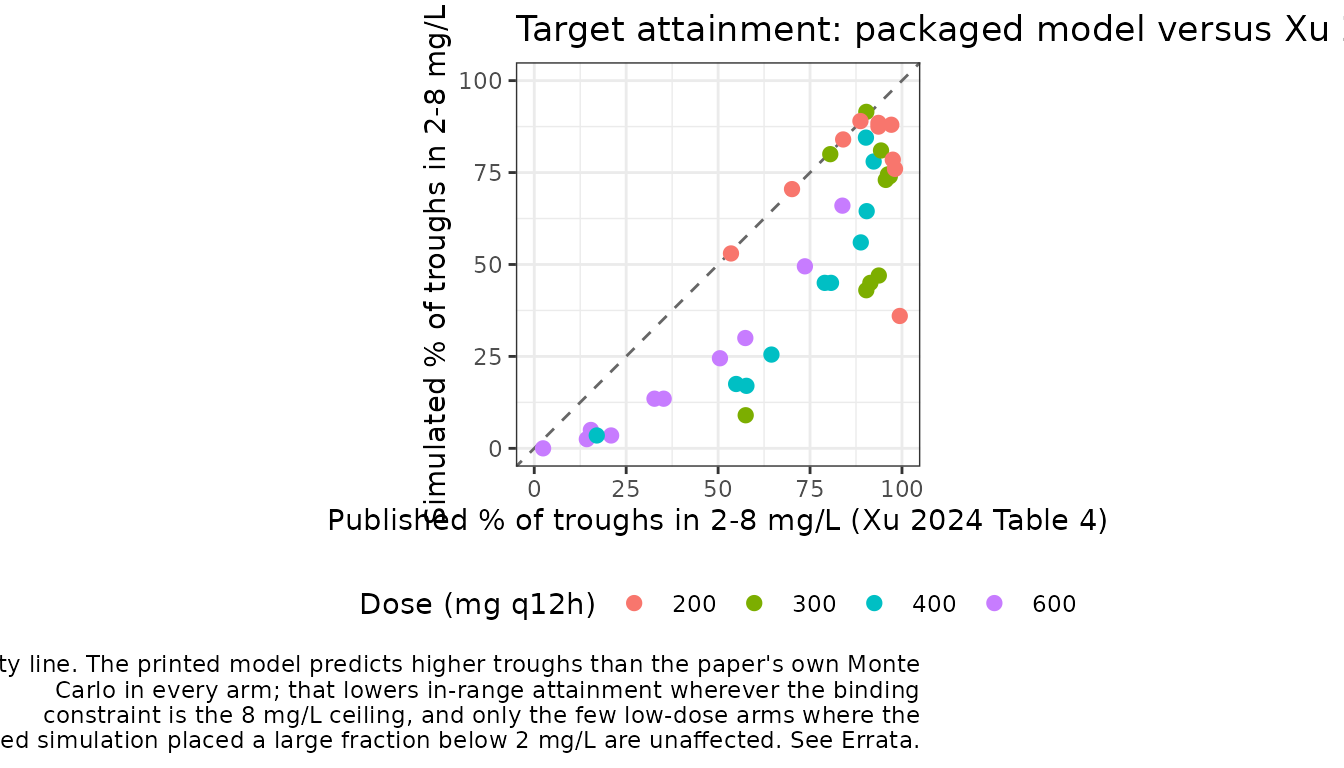

Assumptions and deviations

Structural model, parameters and covariate model are taken verbatim from the paper and reproduce the printed final-model equation to machine precision. Nothing was tuned toward Table 4.
e_age_cl = -0.56 and e_crcl_cl = 0.50 come from the final-model equation on p. 5078, not from Table 3. Table 3 reports the same two coefficients rounded to one decimal place (-0.6 and 0.5); the equation carries two decimal places and is the more precise form. The two are consistent.
omega^2 CL = 0.1 is read as a variance, per the Table 3 footnote (“variance of inter-individual variability of clearance”), giving omega = 0.316, i.e. roughly 32% CV on clearance. The stray “(%)” in that row’s label is inconsistent with the footnote and is read as a table-template artefact.
sigma = 3.4 is read as an additive residual SD in mg/L. The Results text states that “the additive error model was found to best fit the data” and the Table 3 footnote defines sigma as the “square root of residual variability”, so the value sits on the concentration scale. As with omega^2 CL, the “(%)” in the row label contradicts both statements and is treated as an artefact. A proportional reading of 3.4% would be implausibly precise for retrospective therapeutic-drug-monitoring data.
No inter-individual variability on volume of distribution. The printed equation carries exp(eta_CL) on clearance only and V (L) = 57.1 has no random-effect term; Table 3 reports no omega^2 V. This is encoded faithfully rather than adding an eta the paper did not estimate.
CRCL is carried as the raw Cockcroft-Gault value in mL/min, not the register’s canonical BSA-normalized mL/min/1.73 m^2 form, because the paper’s Methods specify Cockcroft-Gault with no BSA step. This is the same documented deviation as Tsuji_2017_linezolid.R, Delattre_2010_amikacin.R and Wada_2023_sparsentan.R.
WT is documented in covariatesDataExcluded, not covariateData. The paper screened body weight as a covariate on clearance and rejected it, so it is preserved as provenance without being referenced in model().
Steady state is requested with ss = 1 / ii = 12 rather than by dosing forward. In the low-CrCL, low-eta corner of this cohort the terminal half-life approaches 50 h, so an explicit multiple-dose run-in would need to be several hundred hours long to be within a percent of steady state. The paper does not state how long its own simulated regimens ran before the trough was read.
The virtual cohort is the paper’s Monte Carlo covariate grid, not a resampled patient population. Xu 2024’s Table 4 fixes age and CrCL at discrete values per arm rather than sampling them, so age and CrCL carry no distribution here and clearance varies only through eta_CL. Cohort size is 200 per arm versus the paper’s 1000 virtual individuals, giving a Monte Carlo standard error of roughly 3.5 percentage points on each probability. That is far smaller than the discrepancy documented below.
Population metadata is the PPK cohort’s own. Every demographic figure in population comes from supplementary Table S1 (n = 166), not from the companion pharmacodynamic study’s n = 81 arm.
No published NCA table exists to compare against. Xu 2024 reports no Cmax / Tmax / AUC / half-life values, so the PKNCA section is gated against the exact one-compartment identity Cav,ss = Dose / (tau * CL) instead of against published NCA numbers, and the Table 4 attainment probabilities carry the published-value comparison.

Quantifying the Table 4 discrepancy

The comparison above shows Table 4 is not reproducible from the paper’s own printed model. The chunk below characterises the discrepancy, so that every number quoted in the Errata that follows is computed here rather than asserted in prose. Each candidate explanation is tested and either quantified or ruled out.

# Closed-form steady-state trough for a 1-compartment model with a constant-rate
# infusion. Agreement with rxode2 is asserted below, so this can be used to
# explore counterfactuals cheaply without re-solving the ODE model.
cmin_ss_cf <- function(dose, Tinf, tau, CL, V) {
  kel <- CL / V
  rate <- dose / Tinf
  cend <- (rate / (V * kel)) * (1 - exp(-kel * Tinf)) / (1 - exp(-kel * tau))
  cend * exp(-kel * (tau - Tinf))
}
cl_printed <- function(age, crcl) 2.7 * (age / 82)^-0.56 * (crcl / 42.0)^0.50

# Trough after the nth dose (not yet at steady state), by superposition.
trough_dose_n <- function(dose, Tinf, tau, CL, V, n) {
  kel <- CL / V
  rate <- dose / Tinf
  cend1 <- (rate / (V * kel)) * (1 - exp(-kel * Tinf))
  cend1 * (1 - exp(-n * kel * tau)) / (1 - exp(-kel * tau)) *
    exp(-kel * (tau - Tinf))
}

arms600 <- published_pta |>
  dplyr::filter(dose_mg == 600) |>
  dplyr::mutate(
    CL           = cl_printed(AGE, CRCL),
    cmin_printed = cmin_ss_cf(600, t_inf, tau, CL, 57.1),
    p_below      = pub_below / 100,
    p_below8     = (pub_below + pub_in) / 100
  )

# Gate the closed form against the rxode2 solution of the packaged model: the
# end-of-interval concentration of the typical-value (eta = 0) simulation must
# equal cmin_ss_cf() for the same covariates and dose.
cf_gate <- sim_typical |>
  dplyr::filter(time == tau) |>
  dplyr::mutate(
    cmin_rxode2 = Cc,
    cmin_closed = cmin_ss_cf(dose_mg, t_inf, tau, cl_printed(AGE, CRCL), 57.1)
  )
stopifnot(
  nrow(cf_gate) == nrow(arms),
  max(abs(cf_gate$cmin_rxode2 - cf_gate$cmin_closed)) < 1e-8
)

# Table 4 prints "0.0%" for the below-2 cell in half of the 600 mg arms, so a
# per-arm two-point (mu, sigma) solve is only identified where that cell is
# non-zero. The claim under test -- a UNIFORM offset with a COMMON dispersion --
# is therefore fitted globally: two parameters (a trough ratio k applied to every
# arm's printed trough, and one log-scale sigma) against all 20 independent
# published probabilities of the ten 600 mg arms.
ln_objective <- function(par, dat) {
  mu <- log(exp(par[1]) * dat$cmin_printed)
  s <- exp(par[2])
  sum((pnorm((log(2) - mu) / s) - dat$p_below)^2 +
        (pnorm((log(8) - mu) / s) - dat$p_below8)^2)
}
ln_fit <- optim(
  c(log(0.73), log(0.44)), ln_objective, dat = arms600,
  method = "Nelder-Mead", control = list(reltol = 1e-14, maxit = 1e5)
)
err_k <- exp(ln_fit$par[1])
err_sigma <- exp(ln_fit$par[2])

# How well does that two-parameter description reproduce Table 4?
mu_fit <- log(err_k * arms600$cmin_printed)
pred_in <- 100 * (pnorm((log(8) - mu_fit) / err_sigma) -
                    pnorm((log(2) - mu_fit) / err_sigma))
err_max_fit <- max(abs(pred_in - arms600$pub_in))
err_rmse_fit <- sqrt(mean((pred_in - arms600$pub_in)^2))

# Per-arm exact two-point solve, where the below-2 cell is informative.
informative <- arms600 |> dplyr::filter(pub_below >= 0.1)
sig_arm <- (log(8) - log(2)) /
  (qnorm(informative$p_below8) - qnorm(informative$p_below))
mu_arm <- log(2) - qnorm(informative$p_below) * sig_arm
err_ratio_arm <- exp(mu_arm) / informative$cmin_printed

# Candidate 1: a higher clearance. Because tau is close to one half-life here,
# the trough is MORE than reciprocally sensitive to CL, so the naive 1/k reading
# overstates the implied clearance change.
err_cl_mult <- uniroot(
  function(m) {
    mean(cmin_ss_cf(600, t_inf, tau, arms600$CL * m, 57.1) / arms600$cmin_printed) - err_k
  },
  c(1, 4)
)$root
err_cl_mult_naive <- 1 / err_k

# Candidate 2: a different volume of distribution. Ruled out if the V required
# to hit the fitted median varies across arms.
err_v_needed <- vapply(
  seq_len(nrow(arms600)),
  function(i) {
    uniroot(
      function(V) cmin_ss_cf(600, t_inf, tau, arms600$CL[i], V) - err_k * arms600$cmin_printed[i],
      c(1, 400)
    )$root
  },
  numeric(1)
)

# Candidate 3: the trough read before steady state. Ruled out if the dose number
# required to hit the fitted ratio varies across arms.
err_n_needed <- vapply(
  seq_len(nrow(arms600)),
  function(i) {
    uniroot(
      function(n) {
        trough_dose_n(600, t_inf, tau, arms600$CL[i], 57.1, n) /
          arms600$cmin_printed[i] - err_k
      },
      c(0.2, 60)
    )$root
  },
  numeric(1)
)

# Candidate 4: Table 4 reports simulated observations rather than individual
# predictions, i.e. the additive residual error is layered on.
set.seed(20241108)
cl_draws <- arms600$CL[1] * exp(rnorm(2e5, 0, sqrt(0.1)))
ipred_draws <- cmin_ss_cf(600, t_inf, tau, cl_draws, 57.1)
err_ipred_below2 <- 100 * mean(ipred_draws < 2)
err_obs_below2 <- 100 * mean(ipred_draws + rnorm(length(ipred_draws), 0, 3.4) < 2)

tibble::tibble(
  Quantity = c(
    "Fitted uniform trough ratio k (published / printed)",
    "Fitted common log-scale sigma",
    "Table 3 sigma for comparison, sqrt(0.1)",
    "Implied IIV variance, sigma^2",
    "Max |error| of the 2-parameter fit to Table 4 % in 2-8 (pp)",
    "RMSE of the 2-parameter fit (pp)",
    "Per-arm ratio, range over identified arms",
    "Per-arm sigma, range over identified arms",
    "CL multiplier consistent with ratio k",
    "CL multiplier under a naive 1/k reading",
    "V (L) required per arm to explain the offset instead",
    "Dose number required per arm to explain the offset instead",
    "% below 2 mg/L, CrCL 90 arm, individual predictions",
    "% below 2 mg/L, CrCL 90 arm, with additive SD 3.4 mg/L",
    "% below 2 mg/L, CrCL 90 arm, Table 4"
  ),
  Value = c(
    sprintf("%.3f", err_k),
    sprintf("%.3f", err_sigma),
    sprintf("%.3f", sqrt(0.1)),
    sprintf("%.3f", err_sigma^2),
    sprintf("%.1f", err_max_fit),
    sprintf("%.1f", err_rmse_fit),
    sprintf("%.3f - %.3f", min(err_ratio_arm), max(err_ratio_arm)),
    sprintf("%.3f - %.3f", min(sig_arm), max(sig_arm)),
    sprintf("x %.3f (+%.0f%%)", err_cl_mult, 100 * (err_cl_mult - 1)),
    sprintf("x %.3f (+%.0f%%)", err_cl_mult_naive, 100 * (err_cl_mult_naive - 1)),
    sprintf("%.0f - %.0f (not constant)", min(err_v_needed), max(err_v_needed)),
    sprintf("%.2f - %.2f (not constant, non-integer)", min(err_n_needed), max(err_n_needed)),
    sprintf("%.1f", err_ipred_below2),
    sprintf("%.1f", err_obs_below2),
    "0.9"
  )
) |>
  knitr::kable(
    caption = paste(
      "Characterisation of the discrepancy between Xu 2024 Table 4 and the",
      "paper's own printed final model, over the ten 600 mg q12h arms.",
      "A single trough ratio plus a single log-scale sigma reproduces the",
      "published table closely; no alternative reading of the printed model",
      "does."
    )
  )

Characterisation of the discrepancy between Xu 2024 Table 4 and the paper’s own printed final model, over the ten 600 mg q12h arms. A single trough ratio plus a single log-scale sigma reproduces the published table closely; no alternative reading of the printed model does.
Quantity	Value
Fitted uniform trough ratio k (published / printed)	0.731
Fitted common log-scale sigma	0.431
Table 3 sigma for comparison, sqrt(0.1)	0.316
Implied IIV variance, sigma^2	0.186
Max \|error\| of the 2-parameter fit to Table 4 % in 2-8 (pp)	1.8
RMSE of the 2-parameter fit (pp)	0.7
Per-arm ratio, range over identified arms	0.712 - 0.748
Per-arm sigma, range over identified arms	0.458 - 0.511
CL multiplier consistent with ratio k	x 1.258 (+26%)
CL multiplier under a naive 1/k reading	x 1.368 (+37%)
V (L) required per arm to explain the offset instead	21 - 36 (not constant)
Dose number required per arm to explain the offset instead	1.35 - 3.82 (not constant, non-integer)
% below 2 mg/L, CrCL 90 arm, individual predictions	0.5
% below 2 mg/L, CrCL 90 arm, with additive SD 3.4 mg/L	8.2
% below 2 mg/L, CrCL 90 arm, Table 4	0.9

Errata and unresolved source issues

Table 4 is not reproducible from the paper’s own final model. This is the substantive finding of this validation; the figures quoted here come from the chunk above. Working from the printed model (one compartment, CL = 2.7 * (age/82)^-0.56 * (CrCL/42.0)^0.50, V = 57.1 L, 1 h infusion, tau = 12 h), the typical steady-state trough at age 80 and CrCL 90 mL/min is 8.2 mg/L and at age 80 and CrCL 15 mL/min it is 26.0 mg/L; the simulated medians in the attainment table above (8.0 and 26.3 mg/L) agree with those closed-form values. Table 4 reports 73.6% and 2.4% of troughs inside 2-8 mg/L for those two arms, far more exposure-favourable than the printed model gives. Describing Table 4’s ten 600 mg arms with just two parameters – one trough ratio applied to every arm, and one common log-scale sigma – reproduces every published in-range probability to within 1.8 percentage points (RMSE 0.7 pp). That fit is the substance of the finding: the arm-to-arm spacing of the published probabilities matches the printed covariate model closely, so the covariate exponents and centering values are right, but the whole distribution sits at a uniform 0.73 of the printed model’s predicted trough, with a dispersion of sigma = 0.43 on the log scale rather than the sqrt(0.1) = 0.316 Table 3 reports. Read as a clearance difference, that offset corresponds to a clearance 26% higher than the printed 2.7 L/h, and to an IIV variance nearer 0.19 than 0.10. Note that the offset is not simply the reciprocal of the trough ratio, which would suggest 37%: with tau close to one half-life the trough falls faster than reciprocally in clearance, so the naive reading overstates the implied change. No alternative reading of the printed model recovers Table 4 – a different volume of distribution cannot produce a uniform trough offset (it would require V to range from 21 to 36 L across the arms), and neither can a pre-steady-state read time (it would require a different, non-integer dose number per arm, ranging from 1.3 to 3.8). The consistency of a single offset and a single sigma across all ten arms indicates the paper’s simulation used the right structure with different numbers, not that the printed equation is mis-transcribed here. The printed model is what is packaged, per the standing rule against tuning parameters to match a validation target.
The residual error is not carried into the published PTA. Table 4’s spread is consistent with a purely lognormal, IIV-driven trough distribution. Layering the additive residual SD of 3.4 mg/L on top of the individual predictions would put 8.2% of the CrCL 90 / 600 mg arm below 2 mg/L, against the 0.9% Table 4 reports; the individual predictions alone give 0.5%, much closer to the published figure. Table 4 therefore reports individual predicted troughs, not simulated observations. The comparison in this vignette follows that convention and uses Cc (the individual prediction) rather than a residual-error-perturbed simulated observation. Note that this makes the published table even harder to reconcile: residual error would widen the distribution toward the fitted sigma of 0.43, but it moves the below-2 tail the wrong way.
sigma and omega^2 CL row labels in Table 3 carry a spurious “(%)” that contradicts the table’s own footnote definitions and the Results text. Resolved as described under Assumptions above.
The supplement was retrieved and contains no final-model parameter. The supplement (get_supplementary_file.php?f=474470.docx from the Dovepress landing page; the EuropePMC supplementaryFiles endpoint for PMC11561734 returns HTTP 200 with 447 kB of the article’s own figure renderings DDDT-18-5073-g0001..g0004 and no supplement, so a 200 with real bytes is not evidence a supplement was found) holds the bioanalytical methods, Table S1 and Table S2. Every final estimate, covariate coefficient and centering value remains in Table 3 or the p. 5078 equation. Table S1 supplies the PPK cohort’s own baseline characteristics, used throughout above. Table S2 is the covariate hypothesis-testing path, and it is narrower than the Methods describe: the Methods specify stepwise forward inclusion followed by backward elimination over a set of “potential covariates”, but Table S2 tabulates only a basic model (OFV 1327.8), a full covariate model carrying CL-CrCL and CL-age (1266.5), and the two backward-elimination steps (+6.9 removing CL-age, +50.7 removing CL-CrCL, both P < 0.01). No forward-inclusion step and no rejected candidate is tabulated, so the rejection of body weight – the one screened covariate the paper names – rests on the Discussion prose alone and cannot be checked against an OFV. The covariates that were screened and rejected besides weight are not recoverable from any source on disk.
The paper’s Discussion misstates the clearance unit as “The estimated linezolid clearance was 2.7 L” (p. 5082); Table 3 and the final-model equation both give L/h. Read as a typographical slip.
No erratum or corrigendum was located for this article.