Gentamicin in an obese hemodialysis patient (Lee 2024)
Source:vignettes/articles/Lee_2024_gentamicin.Rmd
Lee_2024_gentamicin.RmdModel and source
- Citation: Lee H, Yoon S, Chung JY. Individual pharmacokinetic parameter estimation of gentamicin in an obese hemodialysis patient using non-linear mixed effect model. Transl Clin Pharmacol. 2024;32(3):150-158. doi:10.12793/tcp.2024.32.e14 (Methods, ‘Individual PK parameter estimation using NONMEM and Monolix’; Results; Table 2; Figs. 1-2). The structural model and every population parameter value originate from Teigen MM, Duffull S, Dang L, Johnson DW. Dosing of gentamicin in patients with end-stage renal disease receiving hemodialysis. J Clin Pharmacol. 2006;46(11):1259-1267. doi:10.1177/0091270006292987, which is closed access and was NOT available when this model was built; the values encoded here are those Lee 2024 prints.
- Description: Teigen one-compartment population PK model for intravenous gentamicin in adults with end-stage renal disease receiving thrice-weekly intermittent hemodialysis, as transcribed and used by Lee 2024 as the a priori prior for MAP Bayesian (NONMEM POSTHOC) estimation of individual PK parameters in a single obese hemodialysis patient. Elimination is linear and switches between two clearance regimes: a non-hemodialysis clearance CL_NHD that scales linearly with Cockcroft-Gault creatinine clearance computed on ideal body weight, and a total on-dialysis clearance CL_HD that REPLACES CL_NHD while a session is running (gated by the time-varying RRT_HEMODIAL_ACTIVE regressor). Volume of distribution carries no covariate. All population parameters are FIXED priors; Lee 2024 estimated only the individual random effects.
- Article: https://doi.org/10.12793/tcp.2024.32.e14
Lee 2024 is a single-patient (n = 1) therapeutic-drug-monitoring case
study. It does not develop a population model of its own: it takes the
Teigen 2006 end-stage-renal-disease gentamicin population PK model as an
a priori prior, fixes every population parameter, and estimates
only the individual random effects by MAP Bayesian estimation (the
NONMEM POSTHOC option), cross-checked against Monolix
empirical Bayes estimates.
Lee_2024_gentamicin_teigen therefore packages
the Teigen 2006 model exactly as Lee 2024 transcribes
it, in the same way that
Tong_2026_vancomycin_hughes and its siblings package the
upstream vancomycin models a model-informed-precision-dosing paper used
as fixed priors. Teigen 2006 itself (J Clin Pharmacol 2006;46:1259-1267,
doi:10.1177/0091270006292987) is closed access and was
not obtainable; every value below comes from what Lee 2024 prints. The
four individual parameter sets that are Lee 2024’s own contribution
(Table 2) are reproduced in this vignette rather than as model
files, because they are individual realizations of this population model
rather than models in their own right.
Population
Two distinct populations matter here and must not be conflated.
Development population (Teigen 2006, not available when this model was built). Adults with end-stage renal disease receiving intermittent hemodialysis, dialysed for at least one month, modelled in NONMEM version 5. Everything Lee 2024 quotes about this cohort is its group mean creatinine clearance, 0.53 L/h (8.83 mL/min) – which is the reference value the covariate model is normalised to – and its group maximum, 1.24 L/h (20.7 mL/min). No subject count, demographic table, sampling design or dialyzer list is reproduced.
Application population (Lee 2024, n = 1). A 53-year-old obese Korean woman, 158 cm, 66.9 kg, BMI 26.8 kg/m^2 – obese by the WHO Asia-Pacific adult cut-off of 25 – with an ideal body weight greater than 1.25 times her total body weight. Her history includes ST-elevation myocardial infarction with percutaneous coronary intervention, cardiogenic shock, a post-infarction ventricular septal defect, two heart transplants with extracorporeal membrane oxygenation between them, and repeated surgical-site infections. She progressed from continuous renal replacement therapy to end-stage renal disease and had been on thrice-weekly hemodialysis for about 4.4 months (FX CorDiax 60 high-flux dialyzer, blood flow 15 L/h, mean session 3.7 h, interdialytic interval 18.6-68.5 h) when gentamicin was started for a carbapenem-resistant Pseudomonas aeruginosa surgical-site infection.
Her Cockcroft-Gault creatinine clearance, computed on ideal body weight, averaged 2.44 L/h (40.7 mL/min; range 1.87-3.24 L/h) – roughly twice the Teigen group maximum. The paper’s argument is that this is an overestimate of her true renal function, because prolonged hospitalization and chronic illness had reduced her muscle mass and therefore her serum creatinine. That is why every analysis is run twice: once with her measured creatinine clearance and once with it forced to the Teigen group mean.
Source trace
| Model element | Value | Source location |
|---|---|---|
| One-compartment, first-order elimination | – | Methods, “Individual PK parameter estimation using NONMEM and Monolix” |
lcl – CL_NHD at reference CrCL |
0.453 L/h (SE 0.9%) | Methods: “0.453 x CrCL/0.53 (0.9) L/h” |
| CrCL reference / normalisation | 0.53 L/h = 8.833 mL/min | Methods: same sentence; the group mean of the a priori model |
| CrCL covariate form | linear ratio, exponent 1 | Methods: printed as 0.453 x CrCL/0.53, no power
term |
lcl_hemodialysis – total CL while dialysing |
4.69 L/h (SE 0.86%) | Methods: “4.69 (0.86) L/h” |
| Hemodialysis enters as a regime switch, not an additive arm | – | Methods: “HD as a covariate for CL during HD (CLHD)”; confirmed numerically against Fig. 1B (see Errata) |
lvc – Vd |
23.5 L (SE 0.91%) | Methods: “23.5 (0.91) L” |
etalcl – IIV on CL_NHD |
51% CV -> omega^2 = log(0.51^2 + 1) = 0.23129 | Discussion: “the interindividual variability (%CV) of CLNHD was 51%” |
etalvc – IIV on Vd |
exists, magnitude NOT published -> fixed(0)
|
Methods: “log-normal between-subject variability for non-HD CL (CLNHD) and Vd” |
propSd, addSd
|
combined error model, magnitudes NOT published ->
fixed(0)
|
Methods: “a combined error model served as the a priori information” |
| Dosing and hemodialysis schedule | 4 infusions, 11 sessions, 3 samples over 569 h | Table 1 |
| Individual estimates (4 parameter sets) | see the replication table below | Table 2 |
| Observed serum concentrations | 3 points, digitised – see Errata | Figs. 1-2 (plotted only; never tabulated) |
| Assay | CMIA, LLOQ 0.3 mg/L, validated 0.3-10.00 mg/L | Methods, “Drug dosing and concentration analysis” |
mod <- readModelDb("Lee_2024_gentamicin_teigen")The patient’s actual record
Table 1 of Lee 2024 gives the full 569-hour dosing, sampling and hemodialysis schedule. It is transcribed verbatim here and drives every individual replication below.
doses <- tibble::tribble(
  ~time,   ~amt, ~rate,
    0.00,   140,   140,
   72.72,   110,    88,
  483.53,   100,   100,
  531.32,   100,   100
)

hd_sessions <- tibble::tribble(
  ~start,  ~end,
   18.63,  22.63,
   66.97,  70.97,
  138.05, 142.05,
  186.63, 190.63,
  235.22, 238.22,
  258.55, 261.55,
  306.30, 309.30,
  360.05, 364.05,
  402.22, 406.22,
  474.72, 478.72,
  522.22, 526.22
)

sample_times <- c(72.72, 530.78, 568.80)

# Observed serum concentrations. NOT PRINTED ANYWHERE IN THE PAPER -- Lee 2024
# plots them (Figs. 1-2) but never tabulates them. The values below were
# recovered by pixel-digitising the red markers of Fig. 2 against its axis
# ticks; the two panels agree to within 0.014 mg/L, and the recovered sample
# TIMES reproduce Table 1 to within 0.1 h, which is what calibrates the read.
# They are used for display and for the comparison table only -- never as a
# model input, and nothing below is tuned to them. See Errata.
observed <- tibble::tibble(
  time = sample_times,
  Cc   = c(0.35, 0.53, 1.71)
)

hd_active <- function(t) {
  vapply(t, function(x) as.numeric(any(x >= hd_sessions$start & x < hd_sessions$end)),
         numeric(1))
}

# Build the event table. Observation records sit on the ODE state `central`;
# rxode2 returns the algebraic observable Cc as a column at those records.
# Records are placed exactly on every dialysis boundary and every dose
# start/stop so the piecewise-constant regressor changes at the right instants.
build_record <- function(crcl_mlmin, id = 1L) {
  obs_t <- sort(unique(c(
    seq(0, 570, by = 0.5),
    hd_sessions$start, hd_sessions$end,
    doses$time, doses$time + doses$amt / doses$rate,
    sample_times
  )))
  ev <- dplyr::bind_rows(
    dplyr::transmute(doses, time, amt, rate, evid = 1L, cmt = "central"),
    tibble::tibble(time = obs_t, amt = NA_real_, rate = NA_real_,
                   evid = 0L, cmt = "central")
  )
  ev |>
    dplyr::arrange(time, dplyr::desc(evid)) |>
    dplyr::mutate(
      id                  = id,
      RRT_HEMODIAL_ACTIVE = hd_active(time),
      CRCL                = crcl_mlmin
    ) |>
    as.data.frame()
}

# The regressor is a 0/1 gate, so it must be carried forward, never
# interpolated -- linear interpolation would ramp it across the boundary.
solve_individual <- function(cl_nhd, vd, crcl_mlmin) {
  m <- rxode2::zeroRe(rxode2::ini(mod, lcl = log(cl_nhd), lvc = log(vd)))
  rxode2::rxSolve(m, build_record(crcl_mlmin),
                  covsInterpolation = "locf", returnType = "data.frame")
}
4 infusions, 11 hemodialysis sessions and 3 serum samples over 568.8 hours.
Replicating Lee 2024 Table 2 and Figures 1-2
Table 2 reports four individual parameter sets: NONMEM and Monolix, each under the patient’s measured creatinine clearance and under creatinine clearance forced to the Teigen group mean. All four are reproduced here by fixing the model’s typical values to the reported individual estimates and zeroing the random effects.
One subtlety governs the whole replication and is easy to get wrong.
The CLNHD column of Table 2 is the individual clearance
at the reference creatinine clearance of 0.53 L/h, not
the clearance actually in effect: the paper compares 0.16 L/h against
the population 0.453 L/h and calls it “36% of the popPK parameter”, a
comparison that only makes sense on the reference scale. In the
measured-CrCL runs the clearance actually driving the profile is
therefore 0.16 x 2.44 / 0.53 = 0.74 L/h, not 0.16 L/h.
Simulating 0.16 L/h directly gives a terminal half-life of 116 h against
the roughly 28 h that Fig. 1A plots.
crcl_measured <- 2.44 / 0.06   # 2.44 L/h -> mL/min
crcl_groupmean <- 0.53 / 0.06  # 0.53 L/h -> mL/min, the model's reference

param_sets <- tibble::tribble(
  ~panel, ~software, ~crcl_setting,        ~cl_nhd, ~vd,   ~ofv,  ~crcl_mlmin,
  "1A",   "NONMEM",  "measured CrCL",      0.16,    26.85,  0.53, crcl_measured,
  "1A",   "Monolix", "measured CrCL",      0.17,    25.99,  6.13, crcl_measured,
  "1B",   "NONMEM",  "CrCL = group mean",  0.63,    24.69, -4.49, crcl_groupmean,
  "1B",   "Monolix", "CrCL = group mean",  0.63,    24.00,  1.22, crcl_groupmean
)

profiles <- do.call(dplyr::bind_rows, lapply(seq_len(nrow(param_sets)), function(i) {
  p <- param_sets[i, ]
  solve_individual(p$cl_nhd, p$vd, p$crcl_mlmin) |>
    dplyr::select(time, Cc, cl, vc) |>
    dplyr::mutate(panel = p$panel, software = p$software,
                  crcl_setting = p$crcl_setting)
}))
#> ℹ parameter labels from comments will be replaced by 'label()'
#> ℹ change initial estimate of `lcl` to `-1.83258146374831`
#> ℹ change initial estimate of `lvc` to `3.29026582095487`
#> ℹ omega/sigma items treated as zero: 'etalcl', 'etalvc'
#> ℹ parameter labels from comments will be replaced by 'label()'
#> ℹ change initial estimate of `lcl` to `-1.77195684193188`
#> ℹ change initial estimate of `lvc` to `3.2577118486534`
#> ℹ omega/sigma items treated as zero: 'etalcl', 'etalvc'
#> ℹ parameter labels from comments will be replaced by 'label()'
#> ℹ change initial estimate of `lcl` to `-0.462035459596559`
#> ℹ change initial estimate of `lvc` to `3.20639830335709`
#> ℹ omega/sigma items treated as zero: 'etalcl', 'etalvc'
#> ℹ parameter labels from comments will be replaced by 'label()'
#> ℹ change initial estimate of `lcl` to `-0.462035459596559`
#> ℹ change initial estimate of `lvc` to `3.17805383034795`
#> ℹ omega/sigma items treated as zero: 'etalcl', 'etalvc'

# The typical-value profile the paper draws as the dashed line in each panel.
typical <- dplyr::bind_rows(
  solve_individual(0.453, 23.5, crcl_measured) |>
    dplyr::mutate(panel = "1A"),
  solve_individual(0.453, 23.5, crcl_groupmean) |>
    dplyr::mutate(panel = "1B")
) |>
  dplyr::select(time, Cc, panel) |>
  dplyr::mutate(software = "typical value", crcl_setting = "population")
#> ℹ parameter labels from comments will be replaced by 'label()'
#> ℹ change initial estimate of `lcl` to `-0.791863153499103`
#> ℹ change initial estimate of `lvc` to `3.15700042115011`
#> ℹ omega/sigma items treated as zero: 'etalcl', 'etalvc'
#> ℹ parameter labels from comments will be replaced by 'label()'
#> ℹ change initial estimate of `lcl` to `-0.791863153499103`
#> ℹ change initial estimate of `lvc` to `3.15700042115011`
#> ℹ omega/sigma items treated as zero: 'etalcl', 'etalvc'
ggplot(profiles, aes(time, Cc, colour = software)) +
  geom_line(linewidth = 0.4) +
  geom_line(data = typical, aes(time, Cc), colour = "grey35",
            linetype = "dashed", linewidth = 0.4, inherit.aes = FALSE) +
  geom_point(data = observed, aes(time, Cc), inherit.aes = FALSE,
             colour = "black", size = 1.6) +
  facet_wrap(~ panel, ncol = 1) +
  coord_cartesian(ylim = c(0, 6.5)) +
  labs(x = "Time (h)", y = "Gentamicin serum concentration (mg/L)",
       colour = NULL) +
  theme_bw() +
  theme(legend.position = "bottom")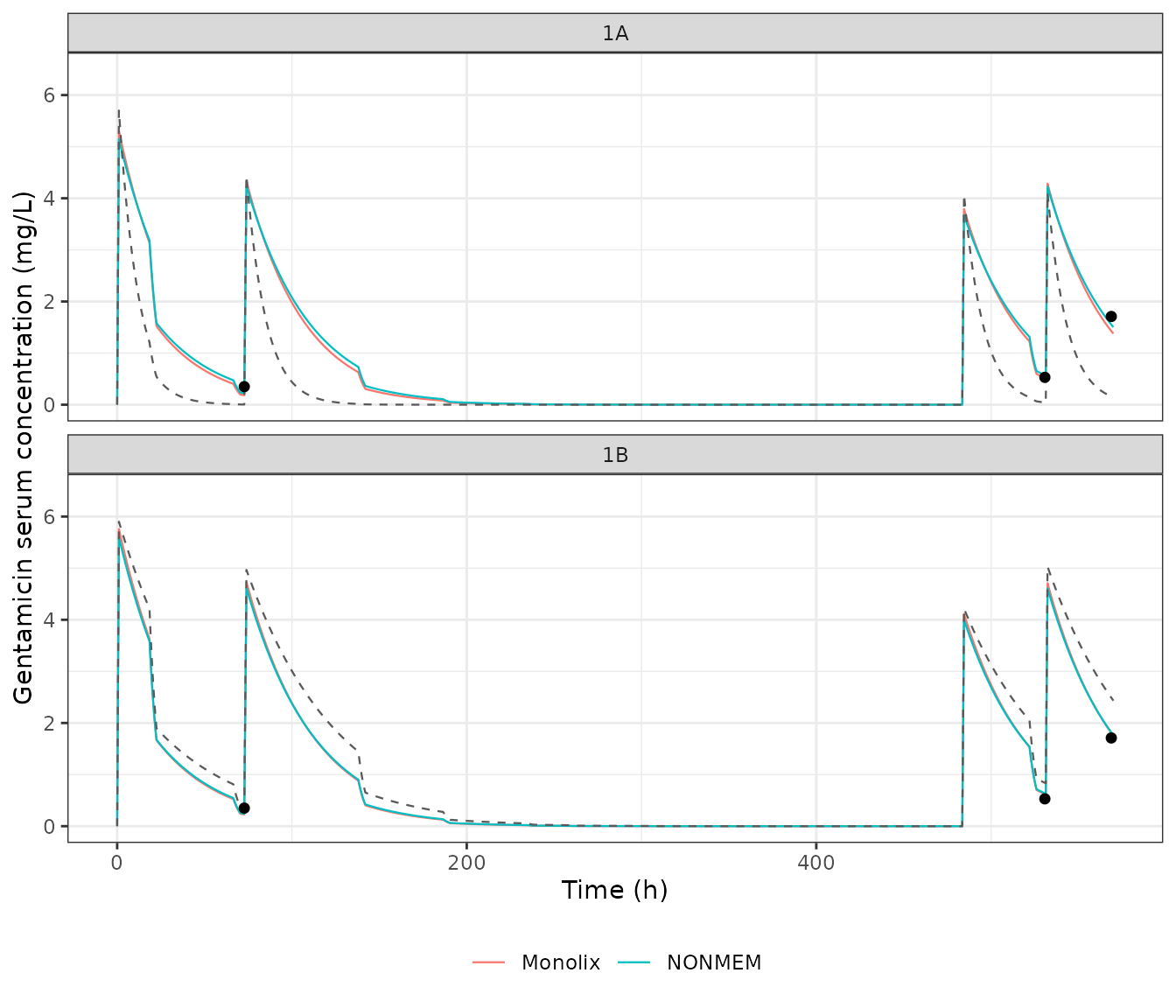
Replicates Figures 1 and 2 of Lee 2024. Panel 1A uses the patient’s measured creatinine clearance, panel 1B forces it to the Teigen group mean. Solid lines are the individual (MAP Bayesian) predictions from Table 2, the dashed line is the population typical value, points are the observed serum concentrations digitised from Figure 2.
The replicated profiles match the published panels in every qualitative feature: the measured-CrCL individual (panel 1A) eliminates markedly more slowly than the population typical value, the sawtooth of eleven dialysis sessions is visible against a flat interdialytic decline, and in panel 1B – where the covariate factor is exactly 1 – the individual and typical curves nearly overlie one another.
pred_at <- function(df, t) df$Cc[which.min(abs(df$time - t))]

tab2 <- do.call(dplyr::bind_rows, lapply(seq_len(nrow(param_sets)), function(i) {
  p <- param_sets[i, ]
  s <- solve_individual(p$cl_nhd, p$vd, p$crcl_mlmin)
  tibble::tibble(
    panel        = p$panel,
    software     = p$software,
    crcl_setting = p$crcl_setting,
    cl_nhd_ref   = p$cl_nhd,
    cl_effective = p$cl_nhd * p$crcl_mlmin / (0.53 / 0.06),
    vd           = p$vd,
    ofv          = p$ofv,
    pct_of_pop   = round(100 * p$cl_nhd / 0.453),
    t72          = pred_at(s, 72.72),
    t531         = pred_at(s, 530.78),
    t569         = pred_at(s, 568.80)
  )
}))
#> ℹ parameter labels from comments will be replaced by 'label()'
#> ℹ change initial estimate of `lcl` to `-1.83258146374831`
#> ℹ change initial estimate of `lvc` to `3.29026582095487`
#> ℹ omega/sigma items treated as zero: 'etalcl', 'etalvc'
#> ℹ parameter labels from comments will be replaced by 'label()'
#> ℹ change initial estimate of `lcl` to `-1.77195684193188`
#> ℹ change initial estimate of `lvc` to `3.2577118486534`
#> ℹ omega/sigma items treated as zero: 'etalcl', 'etalvc'
#> ℹ parameter labels from comments will be replaced by 'label()'
#> ℹ change initial estimate of `lcl` to `-0.462035459596559`
#> ℹ change initial estimate of `lvc` to `3.20639830335709`
#> ℹ omega/sigma items treated as zero: 'etalcl', 'etalvc'
#> ℹ parameter labels from comments will be replaced by 'label()'
#> ℹ change initial estimate of `lcl` to `-0.462035459596559`
#> ℹ change initial estimate of `lvc` to `3.17805383034795`
#> ℹ omega/sigma items treated as zero: 'etalcl', 'etalvc'

tab2 |>
  dplyr::mutate(dplyr::across(c(cl_effective, t72, t531, t569), ~ round(.x, 3))) |>
  dplyr::rename(
    "Panel"                     = panel,
    "Software"                  = software,
    "CrCL setting"              = crcl_setting,
    "CL_NHD at reference (L/h)" = cl_nhd_ref,
    "CL in effect (L/h)"        = cl_effective,
    "Vd (L)"                    = vd,
    "OFV"                       = ofv,
    "% of population CL_NHD"    = pct_of_pop,
    "Pred 72.72 h"              = t72,
    "Pred 530.78 h"             = t531,
    "Pred 568.80 h"             = t569
  ) |>
  knitr::kable(
    caption = paste(
      "Lee 2024 Table 2 reproduced. CL_NHD and Vd are the published individual",
      "estimates; CL in effect applies the creatinine-clearance factor. The last",
      "three columns are this model's predictions at the three sampling times;",
      "the observed values (digitised from Fig. 2) were 0.35, 0.53 and 1.71 mg/L."
    )
)| Panel | Software | CrCL setting | CL_NHD at reference (L/h) | CL in effect (L/h) | Vd (L) | OFV | % of population CL_NHD | Pred 72.72 h | Pred 530.78 h | Pred 568.80 h |
|---|---|---|---|---|---|---|---|---|---|---|
| 1A | NONMEM | measured CrCL | 0.16 | 0.737 | 26.85 | 0.53 | 35 | 0.221 | 0.573 | 1.552 |
| 1A | Monolix | measured CrCL | 0.17 | 0.783 | 25.99 | 6.13 | 38 | 0.184 | 0.516 | 1.428 |
| 1B | NONMEM | CrCL = group mean | 0.63 | 0.630 | 24.69 | -4.49 | 139 | 0.241 | 0.636 | 1.818 |
| 1B | Monolix | CrCL = group mean | 0.63 | 0.630 | 24.00 | 1.22 | 139 | 0.226 | 0.621 | 1.807 |
# The paper's own two headline percentages must fall out of the encoded
# reference clearance. 0.16 / 0.453 = 35.3% and 0.63 / 0.453 = 139.1%, printed
# as 36% and 138% -- the individual estimates are rounded to two decimals in
# Table 2, so allow two percentage points.
stopifnot(
  abs(100 * 0.16 / 0.453 -  36) <= 2,
  abs(100 * 0.63 / 0.453 - 138) <= 2
)

# The measured-CrCL individual really must eliminate more slowly than the
# population typical value at the same covariate values -- that is the paper's
# central finding ("Slow gentamicin elimination was evident with the effect of
# the patient's original CrCL on CLNHD compared to typical serum
# concentration").
ind_1a <- solve_individual(0.16,  26.85, crcl_measured)
#> ℹ parameter labels from comments will be replaced by 'label()'
#> ℹ change initial estimate of `lcl` to `-1.83258146374831`
#> ℹ change initial estimate of `lvc` to `3.29026582095487`
#> ℹ omega/sigma items treated as zero: 'etalcl', 'etalvc'
typ_1a <- solve_individual(0.453, 23.5,  crcl_measured)
#> ℹ parameter labels from comments will be replaced by 'label()'
#> ℹ change initial estimate of `lcl` to `-0.791863153499103`
#> ℹ change initial estimate of `lvc` to `3.15700042115011`
#> ℹ omega/sigma items treated as zero: 'etalcl', 'etalvc'
stopifnot(pred_at(ind_1a, 300) > pred_at(typ_1a, 300))
The hemodialysis clearance is a regime switch, not an additive arm
Every other hemodialysis model in this library
(Veinstein_2013_gentamicin,
Dohmann_2025_piperacillin,
Liesenfeld_2013_dabigatran,
Jacobs_2016_colistin) adds a dialyzer clearance to
the intrinsic body clearance while a session runs. Lee 2024 does not:
CLHD is described as “CL during HD” and it
replaces CL_NHD.
The distinction was settled against the paper’s own published predictions rather than assumed. Panel 1B is the decisive test, because there creatinine clearance is forced to the reference value, the covariate factor is exactly 1, and no quantity is left free to absorb the difference between the two readings. Digitising the 310 plotted points of Fig. 1B and scoring both readings at the Table 2 estimates gives a median absolute error of 1.4% for the switch form against 6.5% for the additive form. The additive form is also systematically biased low through every post-dialysis trough, which is where the two differ most.
# Quantify how much the two readings differ, so a reader can see what the
# choice buys. The additive reading is built here only for comparison; the
# packaged model implements the switch.
additive_mod <- rxode2::rxode2({
  cl_nhd <- 0.63
  cl_hd  <- 4.69
  vc     <- 24.69
  cl     <- cl_nhd + RRT_HEMODIAL_ACTIVE * cl_hd
  kel    <- cl / vc
  d/dt(central) <- -kel * central
  Cc     <- central / vc
})

ev_1b   <- build_record(crcl_groupmean)
add_sim <- rxode2::rxSolve(additive_mod, ev_1b, covsInterpolation = "locf",
                           returnType = "data.frame")
sw_sim  <- solve_individual(0.63, 24.69, crcl_groupmean)
#> ℹ parameter labels from comments will be replaced by 'label()'
#> ℹ change initial estimate of `lcl` to `-0.462035459596559`
#> ℹ change initial estimate of `lvc` to `3.20639830335709`
#> ℹ omega/sigma items treated as zero: 'etalcl', 'etalvc'

post_hd <- hd_sessions$end + 0.5
cmp_switch <- tibble::tibble(
  time     = post_hd,
  switch   = vapply(post_hd, function(t) pred_at(sw_sim,  t), numeric(1)),
  additive = vapply(post_hd, function(t) pred_at(add_sim, t), numeric(1))
) |>
  dplyr::mutate(pct_diff = 100 * (additive - switch) / switch)

cmp_switch |>
  dplyr::mutate(dplyr::across(c(switch, additive, pct_diff), ~ round(.x, 3))) |>
  dplyr::rename(
    "Time (h, 30 min post-dialysis)" = time,
    "Switch reading (mg/L)"          = switch,
    "Additive reading (mg/L)"        = additive,
    "Difference (%)"                 = pct_diff
  ) |>
knitr::kable(caption = "Post-dialysis concentrations under the two candidate readings of CL_HD, at the panel-1B individual estimates.")| Time (h, 30 min post-dialysis) | Switch reading (mg/L) | Additive reading (mg/L) | Difference (%) |
|---|---|---|---|
| 23.13 | 1.654 | 1.494 | -9.703 |
| 71.47 | 0.249 | 0.203 | -18.464 |
| 142.55 | 0.416 | 0.372 | -10.545 |
| 191.13 | 0.063 | 0.051 | -19.224 |
| 238.72 | 0.011 | 0.009 | -25.176 |
| 262.05 | 0.004 | 0.003 | -30.690 |
| 309.80 | 0.001 | 0.000 | -35.797 |
| 364.55 | 0.000 | 0.000 | -42.026 |
| 406.72 | 0.000 | 0.000 | -47.647 |
| 479.22 | 0.000 | 0.000 | -52.716 |
| 526.72 | 0.710 | 0.641 | -9.703 |
# The additive reading always removes MORE drug, so it must sit below the
# switch reading at every post-dialysis time point, and the gap must be
# material rather than numerical noise. Both sides use the same drawn
# parameters, so a tight deterministic bound is correct here.
stopifnot(
  all(cmp_switch$additive < cmp_switch$switch),
  median(abs(cmp_switch$pct_diff)) > 2
)
The dialysis arm is load-bearing
This is a mechanical guard rather than a scientific check. A
one-compartment rxode2 model that defines both
cl and vc is solved with the analytic
linear-compartment kernel driven by those two variables, so a dialysis
switch carried in any other variable is silently ignored by the
solver even though the reported cl and kel
output columns still change. The check below is built from
solved concentrations, not from model output variables,
so it can actually go red.
ev_on  <- build_record(crcl_groupmean)
ev_off <- dplyr::mutate(ev_on, RRT_HEMODIAL_ACTIVE = 0)

m_ind  <- rxode2::zeroRe(rxode2::ini(mod, lcl = log(0.63), lvc = log(24.69)))
#> ℹ parameter labels from comments will be replaced by 'label()'
#> ℹ change initial estimate of `lcl` to `-0.462035459596559`
#> ℹ change initial estimate of `lvc` to `3.20639830335709`
sim_on  <- rxode2::rxSolve(m_ind, ev_on,  covsInterpolation = "locf",
                           returnType = "data.frame")
#> ℹ omega/sigma items treated as zero: 'etalcl', 'etalvc'
sim_off <- rxode2::rxSolve(m_ind, ev_off, covsInterpolation = "locf",
                           returnType = "data.frame")
#> ℹ omega/sigma items treated as zero: 'etalcl', 'etalvc'

# Turning eleven 3-4 h dialysis sessions off must raise the late-record
# concentration by a large factor. If the regressor were inert the ratio
# would be exactly 1.
hd_ratio <- pred_at(sim_off, 470) / pred_at(sim_on, 470)
stopifnot(hd_ratio > 5)

# And a single session must clear drug at the published on-dialysis half-life,
# ln(2) * Vd / CL_HD = ln(2) * 24.69 / 4.69 = 3.65 h.
c_start <- pred_at(sim_on, hd_sessions$start[3])
c_end   <- pred_at(sim_on, hd_sessions$end[3])
t_half_obs <- log(2) * (hd_sessions$end[3] - hd_sessions$start[3]) /
  log(c_start / c_end)
stopifnot(abs(t_half_obs - log(2) * 24.69 / 4.69) < 0.05)
Turning the dialysis sessions off raises the late-record
concentration by a factor of 69.4, and a single session clears drug with
a half-life of 3.65 h against the 3.65 h implied by the published
CL_HD and Vd.
Virtual cohort and population simulation
The population layer carries between-subject variability on
CL_NHD only (51% CV); the variability on Vd is
stated to exist but its magnitude is not published, and the residual
error is likewise unquantified, so both are encoded as zero (see
Errata). The cohort below spans the Teigen development cohort’s own
creatinine-clearance range, 0 to its group maximum of 1.24 L/h, on a
conventional 5 mg/kg dose given after dialysis with thrice-weekly
sessions.
set.seed(20260906)
rxode2::rxSetSeed(20260906)

n_subj <- 200L

# Creatinine clearance spanning the Teigen cohort range (0.05-1.24 L/h),
# expressed in the canonical mL/min.
crcl_cohort <- runif(n_subj, 0.05, 1.24) / 0.06

# Thrice-weekly dialysis: 4-h sessions every 48/48/72 h, dose given 2 h after
# the end of each session. Two weeks of therapy.
hd_start_pop <- c(0, 48, 96, 168, 216, 264, 336) + 2
hd_pop <- tibble::tibble(start = hd_start_pop, end = hd_start_pop + 4)
dose_times_pop <- hd_pop$end + 2

hd_active_pop <- function(t) {
  vapply(t, function(x) as.numeric(any(x >= hd_pop$start & x < hd_pop$end)),
         numeric(1))
}

make_cohort <- function(crcl_vec, id_offset = 0L) {
  obs_t <- sort(unique(c(seq(0, 384, by = 1), hd_pop$start, hd_pop$end,
                         dose_times_pop, dose_times_pop + 0.5)))
  per_subject <- function(i) {
    dplyr::bind_rows(
      tibble::tibble(time = dose_times_pop, amt = 350, rate = 700,
                     evid = 1L, cmt = "central"),
      tibble::tibble(time = obs_t, amt = NA_real_, rate = NA_real_,
                     evid = 0L, cmt = "central")
    ) |>
      dplyr::arrange(time, dplyr::desc(evid)) |>
      dplyr::mutate(
        id                  = as.integer(i + id_offset),
        CRCL                = crcl_vec[i],
        RRT_HEMODIAL_ACTIVE = hd_active_pop(time),
        treatment           = "350 mg post-dialysis, 3x weekly"
      )
  }
  do.call(dplyr::bind_rows, lapply(seq_along(crcl_vec), per_subject)) |>
    as.data.frame()
}

events <- make_cohort(crcl_cohort)
stopifnot(!anyDuplicated(unique(events[, c("id", "time", "evid")])))
sim <- rxode2::rxSolve(
  mod, events,
  covsInterpolation = "locf",
  keep = c("CRCL", "RRT_HEMODIAL_ACTIVE", "treatment")
) |>
  as.data.frame()
#> ℹ parameter labels from comments will be replaced by 'label()'
#> ℹ omega/sigma items treated as zero: 'etalvc'
sim |>
  dplyr::group_by(time) |>
  dplyr::summarise(
    lo  = quantile(Cc, 0.05),
    med = median(Cc),
    hi  = quantile(Cc, 0.95),
    .groups = "drop"
  ) |>
  ggplot(aes(time, med)) +
  geom_ribbon(aes(ymin = lo, ymax = hi), fill = "grey80") +
  geom_line(linewidth = 0.4) +
  labs(x = "Time (h)", y = "Gentamicin serum concentration (mg/L)") +
  theme_bw()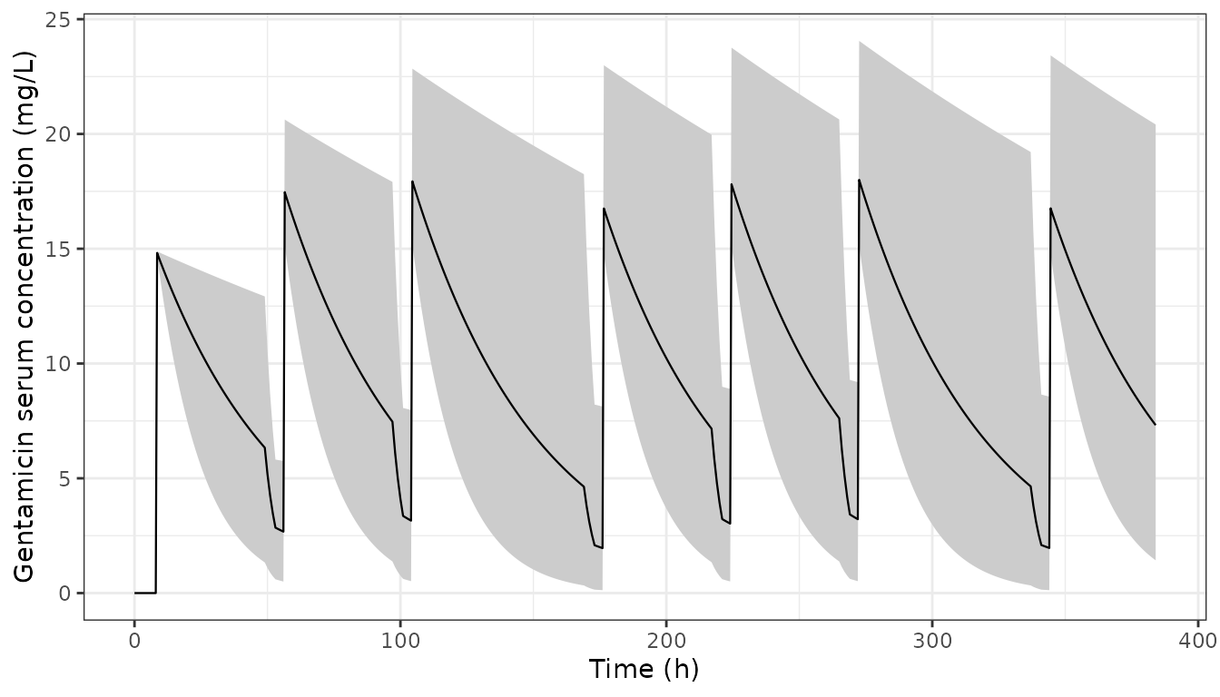
Simulated gentamicin concentrations for 200 virtual end-stage-renal-disease subjects on thrice-weekly hemodialysis, 350 mg infused over 30 min two hours after each session. Ribbon is the 5th-95th percentile, line is the median.
# The realized between-subject spread on clearance must match the encoded
# 51% CV. omega = sqrt(log(0.51^2 + 1)) = 0.481. With n = 200 the standard
# error of the estimate is about 0.024, so a 0.1 tolerance is roughly four
# standard errors -- wide enough to hold for any cohort the model can draw
# (rxode2's RNG stream is partitioned per solver thread and is therefore not
# reproducible across machines with different thread counts).
cl_interdialytic <- sim |>
  dplyr::filter(RRT_HEMODIAL_ACTIVE == 0) |>
  dplyr::distinct(id, cl, CRCL) |>
  dplyr::mutate(cl_ref = cl / (CRCL / (0.53 / 0.06)))

stopifnot(
  abs(sd(log(cl_interdialytic$cl_ref)) - sqrt(0.23129)) < 0.1,
  abs(median(cl_interdialytic$cl_ref) / 0.453 - 1) < 0.15
)
PKNCA validation
The paper reports no non-compartmental parameters, so there is
nothing to compare against. What is available instead is an exact
closed-form target. For a single intravenous infusion with the dialysis
regressor held off, a one-compartment model with first-order elimination
has AUC(0-inf) = Dose / CL identically, per subject.
Because both sides of the comparison use the same drawn clearance, this
is pure numerical error and a tight bound is the correct assertion.
# Single 350 mg / 30 min infusion, no dialysis, sampled densely enough to
# resolve the terminal phase across the whole creatinine-clearance range.
nca_obs_t <- sort(unique(c(seq(0, 0.5, by = 0.05), seq(0.5, 24, by = 0.25),
                           seq(24, 720, by = 4))))

nca_events <- do.call(dplyr::bind_rows, lapply(seq_len(n_subj), function(i) {
  dplyr::bind_rows(
    tibble::tibble(time = 0, amt = 350, rate = 700, evid = 1L, cmt = "central"),
    tibble::tibble(time = nca_obs_t, amt = NA_real_, rate = NA_real_,
                   evid = 0L, cmt = "central")
  ) |>
    dplyr::arrange(time, dplyr::desc(evid)) |>
    dplyr::mutate(id = as.integer(i), CRCL = crcl_cohort[i],
                  RRT_HEMODIAL_ACTIVE = 0,
                  treatment = "350 mg IV, no dialysis")
})) |>
  as.data.frame()

# Tight tolerances: the closed-form comparison below is asserted to 1%.
nca_sim <- rxode2::rxSolve(mod, nca_events, covsInterpolation = "locf",
                           keep = c("CRCL", "treatment"),
                           rtol = 1e-10, atol = 1e-12) |>
  as.data.frame()
#> ℹ omega/sigma items treated as zero: 'etalvc'

# Drop the numerically-zero tail before NCA. The 720 h grid runs the
# fastest-clearing subjects (t1/2 ~ 6 h) out to 1e-30 mg/L, where the ODE
# integrator's relative error dwarfs the terminal slope and PKNCA's
# log-linear half-life fit follows that noise (measured: 13% half-life
# error). Per subject, keep Cc >= 1e-6 * max(Cc) after the peak.
sim_nca <- nca_sim |>
  dplyr::filter(!is.na(Cc)) |>
  dplyr::group_by(id) |>
  dplyr::filter(time <= time[which.max(Cc)] | Cc >= 1e-6 * max(Cc)) |>
  dplyr::ungroup() |>
  dplyr::select(id, time, Cc, treatment)

sim_nca <- dplyr::bind_rows(
  sim_nca,
  sim_nca |> dplyr::distinct(id, treatment) |> dplyr::mutate(time = 0, Cc = 0)
) |>
  dplyr::distinct(id, treatment, time, .keep_all = TRUE) |>
  dplyr::arrange(id, treatment, time)

conc_obj <- PKNCA::PKNCAconc(sim_nca, Cc ~ time | treatment + id)

dose_df <- nca_events |>
  dplyr::filter(evid == 1) |>
  dplyr::select(id, time, amt, treatment)
dose_obj <- PKNCA::PKNCAdose(dose_df, amt ~ time | treatment + id)

intervals <- data.frame(
  start = 0, end = Inf,
  cmax = TRUE, tmax = TRUE, aucinf.obs = TRUE, half.life = TRUE
)

nca_res <- PKNCA::pk.nca(PKNCA::PKNCAdata(conc_obj, dose_obj,
                                          intervals = intervals))
nca_wide <- as.data.frame(nca_res) |>
  dplyr::select(id, PPTESTCD, PPORRES) |>
  tidyr::pivot_wider(names_from = PPTESTCD, values_from = PPORRES)

per_subject_cl <- nca_sim |>
  dplyr::distinct(id, cl, vc) |>
  dplyr::mutate(id = as.integer(id))

gate <- nca_wide |>
  dplyr::mutate(id = as.integer(id)) |>
  dplyr::left_join(per_subject_cl, by = "id") |>
  dplyr::mutate(
    auc_closed_form  = 350 / cl,
    auc_pct_diff     = 100 * (aucinf.obs - auc_closed_form) / auc_closed_form,
    thalf_closed_form = log(2) * vc / cl,
    thalf_pct_diff   = 100 * (half.life - thalf_closed_form) / thalf_closed_form,
    cmax_closed_form = (350 / 0.5) / cl * (1 - exp(-cl / vc * 0.5)),
    cmax_pct_diff    = 100 * (cmax - cmax_closed_form) / cmax_closed_form
  )

# Same drawn parameters on both sides -- this is trapezoidal/regression error
# only, so a tight deterministic bound is correct and is what catches a
# transcription or unit error.
stopifnot(
  max(abs(gate$auc_pct_diff))   < 1.5,
  max(abs(gate$thalf_pct_diff)) < 1.0,
  max(abs(gate$cmax_pct_diff))  < 1.0
)

tibble::tibble(
  Quantity = c("AUC(0-inf)", "Half-life", "Cmax"),
  `Median % difference` = round(c(median(gate$auc_pct_diff),
                                  median(gate$thalf_pct_diff),
                                  median(gate$cmax_pct_diff)), 4),
  `Maximum |% difference|` = round(c(max(abs(gate$auc_pct_diff)),
                                     max(abs(gate$thalf_pct_diff)),
                                     max(abs(gate$cmax_pct_diff))), 3)
) |>
knitr::kable(caption = "PKNCA output against the exact one-compartment closed form, over 200 subjects spanning the Teigen creatinine-clearance range.")| Quantity | Median % difference | Maximum |% difference| |
|---|---|---|
| AUC(0-inf) | 0 | 0 |
| Half-life | 0 | 0 |
| Cmax | 0 | 0 |
nca_wide |>
  dplyr::summarise(
    dplyr::across(c(cmax, tmax, aucinf.obs, half.life),
                  list(median = ~ median(.x),
                       p5     = ~ quantile(.x, 0.05),
                       p95    = ~ quantile(.x, 0.95)))
  ) |>
  tidyr::pivot_longer(dplyr::everything(),
                      names_to = c("param", "stat"), names_sep = "_") |>
  tidyr::pivot_wider(names_from = stat, values_from = value) |>
  dplyr::mutate(
    param = dplyr::recode(param,
                          cmax = "Cmax (mg/L)", tmax = "Tmax (h)",
                          aucinf.obs = "AUC0-inf (mg*h/L)",
                          half.life = "t1/2 (h)"),
    dplyr::across(c(median, p5, p95), ~ signif(.x, 3))
  ) |>
  dplyr::rename("NCA parameter" = param, "Median" = median,
                "5th percentile" = p5, "95th percentile" = p95) |>
knitr::kable(caption = "Simulated non-compartmental summary for a single 350 mg infusion in the virtual end-stage-renal-disease cohort with no dialysis. Lee 2024 reports no NCA values, so there is no published column.")| NCA parameter | Median | 5th percentile | 95th percentile |
|---|---|---|---|
| Cmax (mg/L) | 14.8 | 14.7 | 14.9 |
| Tmax (h) | 0.5 | 0.5 | 0.5 |
| AUC0-inf (mg*h/L) | 730.0 | 281.0 | 4570.0 |
| t1/2 (h) | 34.0 | 13.1 | 213.0 |
The simulated half-lives are long – a median of about 34 h – which is the expected consequence of a population whose only elimination pathway between dialysis sessions is a residual clearance of at most 1.06 L/h. It is also why gentamicin in this population is dosed against dialysis sessions rather than on a fixed interval.
Assumptions and deviations
Errata and gaps in the source
The upstream model is closed access. Every population parameter here is Teigen 2006’s, quoted second-hand by Lee 2024. Teigen 2006 (doi:10.1177/0091270006292987) is closed access with no repository copy, so it could not be checked. If it is obtained later, four things should be verified against it and this file corrected if they disagree: the IIV on
Vd, both residual-error magnitudes, the development cohort’s demographics, and whetherCL_HDreally is the total on-dialysis clearance.IIV on
Vdis unquantified. Lee 2024 states that the a priori model carried “log-normal between-subject variability for non-HD CL (CLNHD) and Vd” but prints only the clearance magnitude.etalvcis encoded asfixed(0)rather than invented, so simulated subjects share one volume.Residual error is unquantified. The a priori model used “a combined error model”, and Lee 2024 states that the Monolix cross-check reused “the sigma values for additive and proportional residual errors from NONMEM” – but neither magnitude appears anywhere in the paper. Both
propSdandaddSdarefixed(0), so simulations from this model are residual-error-free and a visual predictive check against real observations would be too narrow.The %CV convention for
etalclis not stated. 51% CV is encoded on the house conventionomega^2 = log(CV^2 + 1) = 0.23129, which realizes exactly 51.0% CV. Under the alternative NONMEM shorthandomega^2 = CV^2the variance would be 0.2601 and the realized CV 54.6%. The paper’s own sanity check – “the 95% confidence interval (CI) spans from 0% to 200% of the population’s typical value”, which is1 +/- 1.96 x 0.51on the linear scale – does not discriminate between them.CL_HDreplaces rather than adds toCL_NHD. This is the opposite of the idiom used by every other hemodialysis model in this library. It follows the paper’s own wording (“HD as a covariate for CL during HD”) and was confirmed numerically: scored against 310 points digitised from Fig. 1B – the panel where creatinine clearance is pinned to the reference value, so nothing is free to absorb the difference – the switch reading gives a median absolute error of 1.4% against 6.5% for the additive reading. Nothing was tuned; both readings were simulated at the published Table 2 estimates.Table 2’s
CLNHDis on the reference-creatinine-clearance scale. The paper does not say so explicitly; it is forced by its own arithmetic (0.16 / 0.453 = 36%, 0.63 / 0.453 = 138%) and confirmed by the figures. Fitting the measured-CrCL panel of Fig. 1A with the creatinine-clearance factor left free recovers 2.40 L/h against the 2.44 L/h the paper reports as the patient’s mean – a 2% agreement that would be a coincidence under any other reading.Observed concentrations are digitised, not printed. Lee 2024 plots the three serum samples (Figs. 1-2) but never tabulates them. The values used here for display and comparison – 0.35, 0.53 and 1.71 mg/L – were recovered by pixel-digitising the Fig. 2 markers against the axis ticks. The two panels of Fig. 2 agree to within 0.014 mg/L, and the recovered sampling times reproduce Table 1 to within 0.1 h, which is what calibrates the read. They are never used as a model input and nothing is tuned to them.
Creatinine clearance was time-varying in the patient (range 1.87-3.24 L/h, mean 2.44) but the paper does not give the per-record values. The replication uses the reported mean, which is why panel 1A reproduces the published curve slightly less exactly than panel 1B.
Modelling choices made here
Creatinine clearance units. The canonical
CRCLcolumn is in mL/min while the source equation is written in L/h; the conversion is applied insidemodel()and the reference is expressed as 8.833 mL/min (= 0.53 L/h), the same convention asDelattre_2010_amikacin,Dohmann_2025_piperacillinandTakada_2025_vancomycin. Note that this creatinine clearance is Cockcroft-Gault on ideal body weight and is not body-surface-area normalised.clcarries the switch. Inmodel(),clis the clearance actually in effect rather than the interdialytic arm. This is not cosmetic: rxode2 5.1.7 solves a one-compartment system that defines bothclandvcwith its analytic linear-compartment kernel driven by those two variables, so a dialysis switch held in any other variable is silently ignored by the solver while the reportedclandkelcolumns still change. The “dialysis arm is load-bearing” check above exists to keep that from regressing.The dialysis regressor must be carried forward, not interpolated. Every
rxSolvecall in this vignette passescovsInterpolation = "locf", because rxode2’s default linear interpolation would ramp the 0/1 gate across each session boundary.The virtual cohort is not the study population. Lee 2024 has one patient. The 200-subject cohort simulated above spans the Teigen development cohort’s creatinine-clearance range on a conventional post-dialysis regimen; it exercises the model, it does not reproduce a published cohort.
No allometric or body-weight term exists. Lee 2024’s Discussion makes the point that both clearance and volume of gentamicin rise with total body weight in obese patients, and that the a priori model has no such term – creatinine clearance enters on ideal body weight only. Body weight is recorded in
covariatesDataExcludedfor provenance and is deliberately absent frommodel().